Lecture 02: Introduction to Bayesian Statistics

Chun-Hao Yang

Beta-Binomial Model

Beta-Binomial model

Let $X_1, \ldots, X_n \mid p \iid \ber(p)$.
Consider the prior $p \sim \text{Beta}(\alpha, \beta)$ where $\alpha$ and $\beta$ are known.
The posterior distribution of $p$ given $X_1, \ldots, X_n$ is \[ p \mid X_1, \ldots, X_n \sim \text{Beta}\left(\alpha + \sum_{i=1}^n X_i, \beta + n - \sum_{i=1}^n X_i \right). \]

Derivation

Bayes Theorem: \[\begin{align*} \pi(p \mid x) & = \frac{f(x \mid p) \pi(p)}{\int f(x \mid p) \pi(p) dp} = \frac{\text{likelihood} \times \text{prior}}{\text{marginal}}\\ & \propto f(x \mid p) \pi(p) = \text{likelihood} \times \text{prior} \end{align*}\]
The marginal (and other normalizing constants) can be ignored.
The likelihood is \[ f(x_1, \ldots, x_n \mid p) = \prod_{i=1}^n p^{x_i}(1-p)^{1-x_i} = p^{\sum_{i=1}^n x_i}(1-p)^{n - \sum_{i=1}^n x_i}. \]
The prior is \[ \pi(p) = \frac{1}{B(\alpha, \beta)} p^{\alpha-1} (1-p)^{\beta-1} \propto p^{\alpha-1}(1-p)^{\beta - 1}. \]

Derivation

Hence the posterior is \[\begin{align*} \pi(p \mid X_1, \ldots, X_n) & \propto p^{\sum_{i=1}^n x_i}(1-p)^{n - \sum_{i=1}^n x_i} \times p^{\alpha-1}(1-p)^{\beta - 1}\\ & = p^{\alpha + \sum_{i=1}^n x_i - 1}(1-p)^{\beta + n - \sum_{i=1}^n x_i - 1}. \end{align*}\]
Recognizing that this is the kernel of a Beta distribution, the posterior is \[ p \mid X_1, \ldots, X_n \sim \text{Beta}\left(\alpha + \sum_{i=1}^n X_i, \beta + n - \sum_{i=1}^n X_i \right). \]
It’s called Beta-Binomial model since the posterior only depends on $\sum X_i$ and the distribution of $\sum X_i$ is $\bin(n,p)$.

Kernel of a pdf/pmf

The kernel is the form of the pdf or pmf in which any factors that are not functions of any of the variables in the domain are omitted.
Examples:
- Normal: $\exp\left(-\frac{(x-\mu)^2}{2\sigma^2}\right)$
- Gamma: $x^{\alpha-1}\exp(-\beta x)$
- Beta: $x^{\alpha-1}(1-x)^{\beta-1}$
- Poisson: $\frac{\lambda^x}{x!}$
We can use only the kernels to simplify the computation.

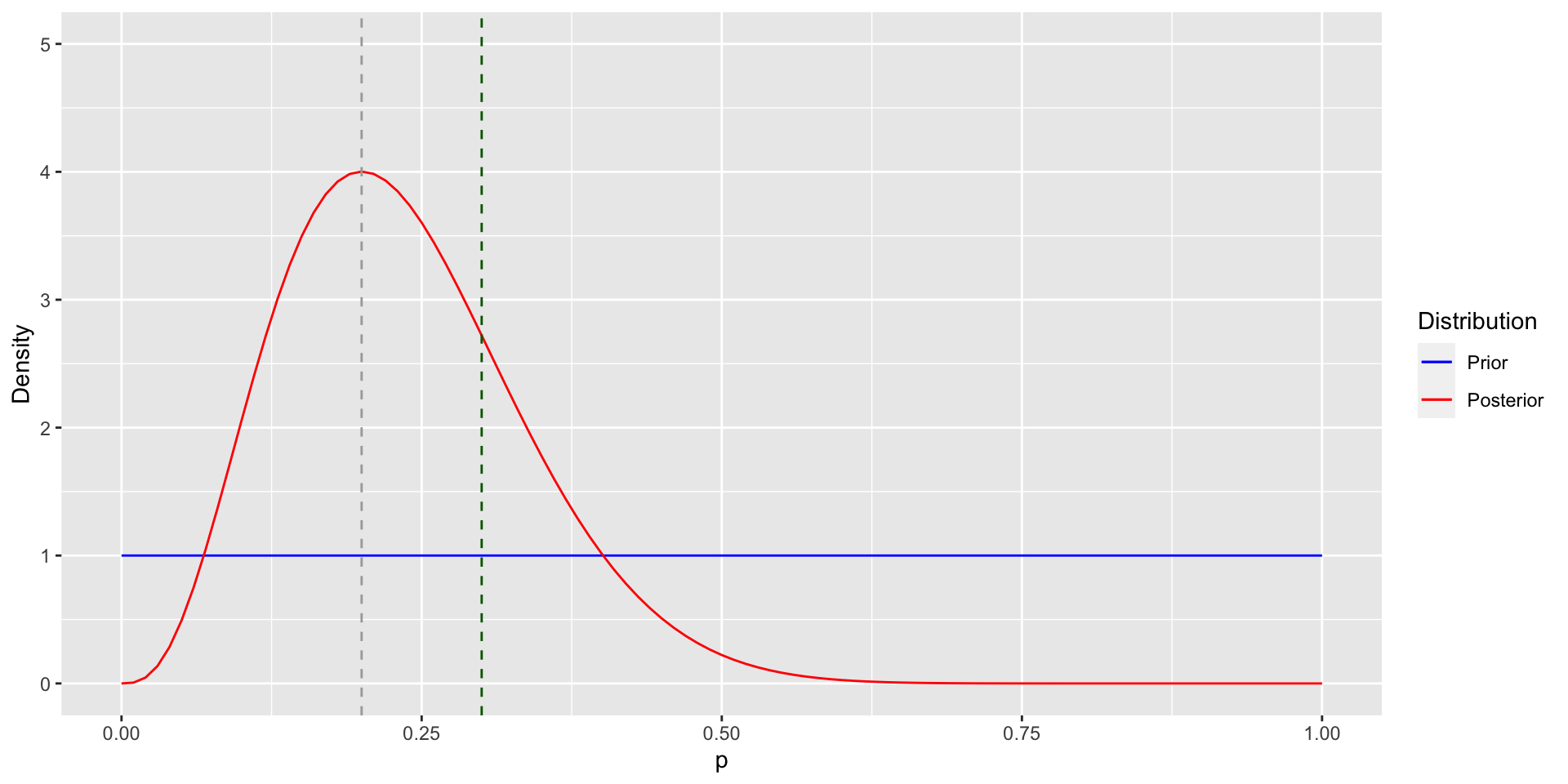
Posterior Distribution

set.seed(2023)
n <- 15
p <- 0.3
X <- rbinom(n, 1, p)
s <- sum(X)
p_mle <- s/n # MLE
print(X)

 [1] 0 0 0 0 0 0 0 0 0 0 1 0 0 1 1

library(ggplot2)
ggplot(data = data.frame(p = c(0, 1)), aes(p)) + 
    lims(x = c(0, 1), y = c(0, 5)) + 
    labs(x = "p", y = "Density") +
    geom_function(fun = dunif, aes(col = "blue")) + 
    geom_function(fun = dbeta, aes(col = "red"), 
                  args = list(shape1 = s + 1, shape2 = n - s + 1)) + 
    geom_vline(xintercept = p_mle, linetype = "dashed", col = "darkgrey") + 
    geom_vline(xintercept = p, linetype = "dashed", col = "darkgreen") + 
    scale_colour_manual(name = "Distribution", 
                        values = c("blue", "red"),
                        labels = c("Prior", "Posterior"))

Posterior Distribution

Posterior Inference

The posterior distribution of $p$ contains much more information than the MLE.
We can use the posterior for:
- Estimation: $\hat{p} = \E(p \mid X_1, \ldots, X_n)$ (posterior mean)
- Prediction: $\P(X_{n+1} = 1 \mid X_1, \ldots, X_n)$
- Interval estimation: Find $(L, U)$ such that $\P(L \leq p \leq U \mid X_1, \ldots, X_n) = 0.95$
In the Beta-Binomial model, an estimate for $p$ is \[ \hat{p} = \E(p \mid X_1, \ldots, X_n) = \frac{\alpha + \sum_{i=1}^n X_i}{\alpha + \beta + n} \] whereas the MLE is $\hat{p}_{\text{MLE}} = \frac{1}{n}\sum_{i=1}^nX_i$.

Maximum-a-posteriori Estimate

The posterior mean is not the only estimate we can obtain from the posterior.
Another commonly used estimator is the maximum-a-posterior (MAP) estimate \[ \hat{p}_{\text{MAP}} = \argmax_{0 < p < 1} \pi(p \mid X_1, \ldots, X_n). \]
Since the mode of $\text{Beta}(\alpha, \beta)$ is $\frac{\alpha-1}{\alpha+\beta-2}$ when $\alpha, \beta > 1$, \[ \hat{p}_{\text{MAP}} = \frac{\alpha -1 + \sum_{i=1}^n X_i}{\alpha + \beta + n - 2}. \]
If $\alpha = \beta = 1$ and $\sum X_i > 1$, then $\hat{p}_{\text{MAP}} = \hat{p}_{\text{MLE}} = \bar{X}$.

Recall: Laplace’s Rule of Succession

Given binary iid random variables $X_1, \ldots, X_n$ with $\sum_{i=1}^n X_i = s$, then \[\P\left(X_{n+1}=1 \mid X_1+\cdots+X_n=s\right)=\frac{s+1}{n+2}.\]

Derivation:

Let $X_1, \ldots, X_n \iid \ber(p)$ and $p \sim \text{Beta}(1,1)$ (the uniform prior).
The posterior is $p \mid X_1 + \cdots + X_n = s \sim \text{Beta}(s + 1, n-s + 1)$.
Assuming $X_{n+1} \sim \ber(p)$ and $X_i$’s are iid conditioned on $p$, \[\begin{align*} \P\left(X_{n+1}=1 \mid \sum X_i=s\right) & = \int \P(X_{n+1}=1 \mid p)\pi\left(p \mid \sum X_i = s\right) dp\\ & = \int p \pi\left(p \mid \sum X_i = s\right) dp = \frac{s+1}{n+2}. \end{align*}\]

Interval Estimation: Credible Interval/Region

For frequentists, it’s called confidence interval/region.
Let $[L(X), U(X)]$ be an interval for $\theta$ based on sample $X$.
$100\times(1-\alpha)\%$ Bayesian Coverage: $\P(L(x) \leq \theta \leq U(x) \mid {\color{magenta}X = x}) = 1-\alpha$.
- describes your information about the location of the true value of $\theta$ after you have observed $X = x$
$100\times(1-\alpha)\%$ Frequentist Coverage: $\P(L(X) \leq \theta \leq U(X) \mid {\color{magenta}\theta}) = 1-\alpha$
- describes the probability that the interval will cover the true value before the data are observed
There are many ways to construct a credible interval:
- Quantile-based method
- Highest posterior density (HPD) region

Quantile-based method

To find a $100\times(1-\alpha)\%$ credible interval for $\theta$:

Find numbers $\theta_{\alpha / 2} < \theta_{1-\alpha / 2}$ such that
1. $\P\left(\theta<\theta_{\alpha/2} \mid X = x\right)=\alpha / 2$;
2. $\P\left(\theta>\theta_{1-\alpha / 2} \mid X = x\right)=\alpha / 2$.
The numbers $\theta_{\alpha / 2}, \theta_{1-\alpha / 2}$ are the $\alpha / 2$ and $1-\alpha / 2$ posterior quantiles of $\theta$, and so \[\begin{align*} \P\left(\theta \in\left[\theta_{\alpha / 2}, \theta_{1-\alpha / 2}\right] \mid X = x\right) & =1-\P\left(\theta \notin\left[\theta_{\alpha / 2}, \theta_{1-\alpha / 2}\right] \mid X = x\right) \\ & =1-\left[\P\left(\theta<\theta_{\alpha / 2} \mid X=x\right)\right.\\ & \qquad \left.+\P\left(\theta>\theta_{1-\alpha / 2} \mid X = x\right)\right] \\ & =1-\alpha. \end{align*}\]

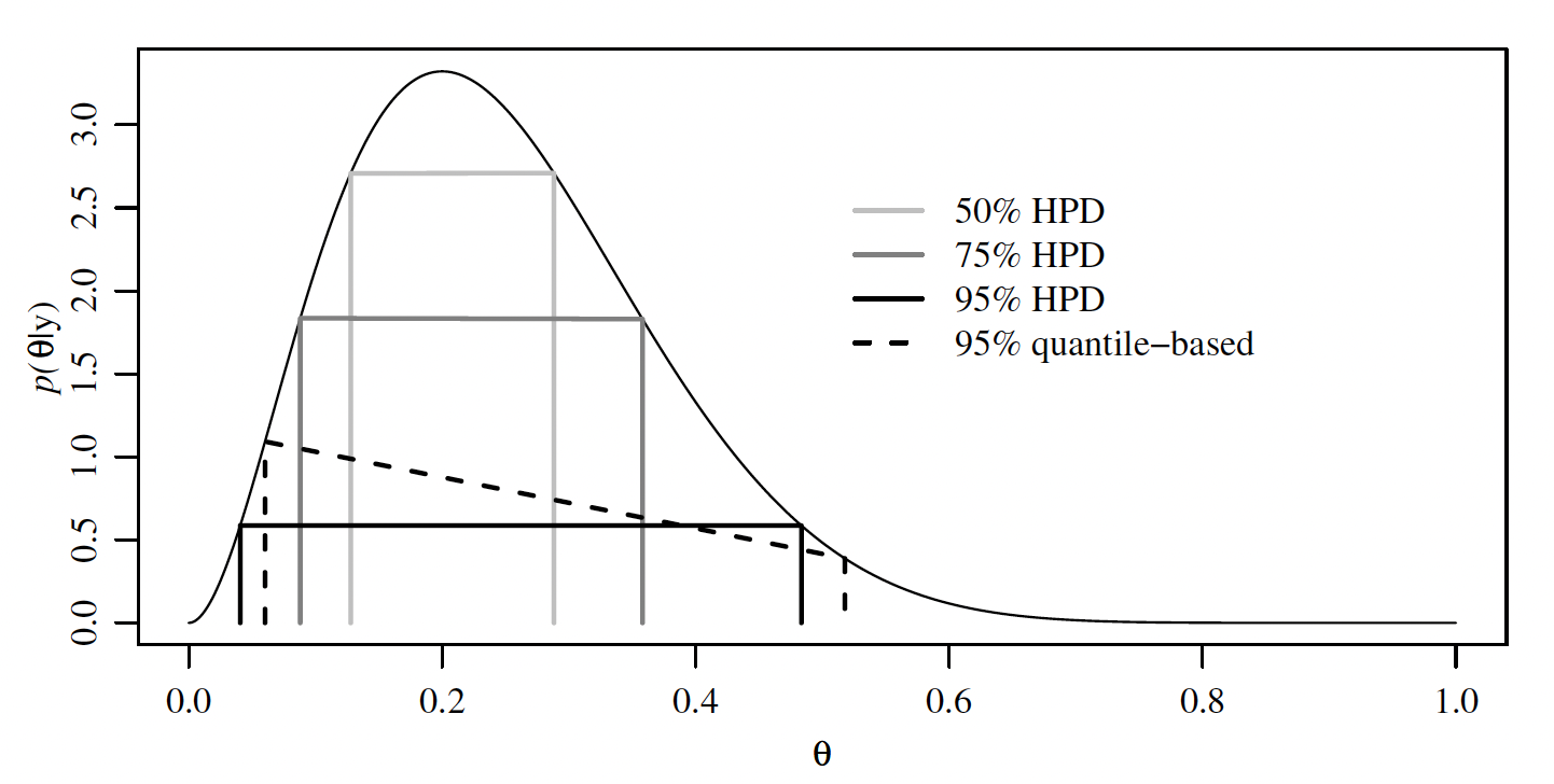
Binomial Example

Suppose we observed $X=2$ from a $\bin(10, p)$. Assume the uniform prior $p$.

alpha <- 1; beta <- 1 # uniform prior
n <- 10; X <- 2 # data

qbeta(c(0.025, 0.975), alpha + X, beta + n - X)

[1] 0.06021773 0.51775585

Highest posterior density (HPD) region

Definition 1 A $100 \times(1-\alpha) \%$ HPD region consists of a subset of the parameter space, $s(x) \subset \Theta$ such that

$\P(\theta \in s(x) \mid X = x)=1-\alpha$;
If $\theta_a \in s(x)$, and $\theta_b \notin s(x)$, then $\pi\left(\theta_a \mid X=x\right)>\pi\left(\theta_b \mid X=x\right)$.

An HPD region might not be an interval if the posterior density is multimodal (having multiple peaks).

Binomial Example

Let’s compute the HPD for the previous example: $\theta \mid X = 2 \sim \text{Beta}(3, 9)$.

library(HDInterval)
hdi(qbeta, 0.95, shape1 = 3, shape2 = 9)

     lower      upper 
0.04055517 0.48372366 
attr(,"credMass")
[1] 0.95

The HPD is narrower than the quantile-based interval.

Wrap-up for the Beta-Binomial model

The Beta-Binomial model: \[\begin{align*} X \mid p & \sim \bin(n,p)\\ p & \sim \text{Beta}(\alpha,\beta)\\ p \mid X & \sim \text{Beta}(\alpha + X, \beta + n - X) \end{align*}\]
Note that the posterior is in the same family of the prior: both of them are in the Beta family.
In this case, the Beta prior is called a conjugate prior for the Binomial model.

Catalog for conjugate priors

Sampling model	Parameter	Prior	Posterior
$X \sim \bin(n, p)$	$p$	$\text{Beta}(\alpha_0, \beta_0)$	$\text{Beta}(\alpha_0 + X, \beta_0+n-X)$
$X \sim N(\mu, \sigma^2)$	$\mu$	$N(\mu_0, \sigma_0^2)$	$N\left(\frac{1}{\frac{1}{\sigma_0^2}+\frac{1}{\sigma^2}}\left(\frac{\mu_0}{\sigma_0^2}+\frac{ X}{\sigma^2}\right),\left(\frac{1}{\sigma_0^2}+\frac{1}{\sigma^2}\right)^{-1}\right)$
$X \sim \text{Poisson}(\lambda)$	$\lambda$	$\text{Gamma}(\alpha_0, \beta_0)$	$\text{Gamma}(\alpha_0 + X, \beta_0+1)$
$X \sim \text{Gamma}(\alpha, \beta)$	$\beta$	$\text{Gamma}(\alpha_0, \beta_0)$	$\text{Gamma}(\alpha_0 + \alpha, \beta_0+X)$
$X \sim \text{NB}(r, p)$	$p$	$\text{Beta}(\alpha_0, \beta_0)$	$\text{Beta}(\alpha_0 + r, \beta_0+X)$

More can be found on Wiki
Exercise: Derive the posterior for the Normal-Normal model.

Real Data Example

2022年，基隆市男女嬰出生數分別為856及731，性別比例為1.171¹（生下男嬰機率為0.5394）。
同年，全台灣男女嬰出生數分別為71,208及66,205，性別比例為1.076（生下男嬰機率為0.5183）
根據統計，全球人類自然出生性別比1.05²（生下男嬰機率為0.5122）。
基隆市自然出生性別比是否高於台灣平均？

Real Data Example

library(tidyverse)
library(knitr)

m <- 856; f <- 731
prior_mean <- c(0.5, 0.5122, 0.5122, 0.5122, 0.5122, 0.5122)
alpha_plus_beta <- c(2, 2, 10, 100, 1000, 10000)
alpha <- prior_mean * alpha_plus_beta
beta <- alpha_plus_beta - alpha

data.frame(alpha, beta, prior_mean) |> 
    mutate(alpha_plus_beta = alpha + beta,
           post_mean = (alpha+m)/(alpha+beta+m+f),
           ratio = post_mean/(1-post_mean),
           post_int = paste0("[", round(qbeta(0.025, alpha + m, beta + f), 3),
                             ", ", round(qbeta(0.975, alpha + m, beta + f), 3), "]")) |>
    select(c(prior_mean, alpha_plus_beta, post_mean, ratio, post_int)) |>
    kable(format = "markdown", digits = 4,
          col.names = c("Prior mean $\\frac{\\alpha}{\\alpha+\\beta}$",
                        "$\\alpha + \\beta$",
                        "Post. mean", "Gender ratio",
                        "Post. 95% Interval"))

Real Data Example

Prior mean $\frac{\alpha}{\alpha+\beta}$	$\alpha + \beta$	Post. mean	Gender ratio	Post. 95% Interval
0.5000	2	0.5393	1.1708	[0.515, 0.564]
0.5122	2	0.5393	1.1708	[0.515, 0.564]
0.5122	10	0.5392	1.1702	[0.515, 0.564]
0.5122	100	0.5378	1.1634	[0.514, 0.562]
0.5122	1000	0.5289	1.1226	[0.51, 0.548]
0.5122	10000	0.5159	1.0658	[0.507, 0.525]

Some follow-up questions

Is the sample size (856+731=1587) large enough?
Which prior? Depend on how strong your prior belief is.
- No prior knowledge $\Rightarrow$ Uniform prior
- Reliable prior information $\Rightarrow$ prior with larger $\alpha+\beta$
With prior information, we can obtain better estimates when the sample size is small:
- For example, think of a really small village in which only two boys and one girl were born last year.
- If we don’t use any prior information, the gender ratio is 2.
What if our prior information cannot be described by a Beta distribution?
- Ex: our prior information indicates a multimodal distribution
- The posterior will be complicated and we need some other methods for posterior inference.

Small Area Estimation (SAE)

The previous example is an example of an SAE problem.

Small area estimation is any of several statistical techniques involving the estimation of parameters for small sub-populations, generally used when the sub-population of interest is included in a larger survey¹.

There is a hierarchical structure in SAE problems:

\[ \text{基隆} \subset \text{台灣} \subset \text{東亞} \subset \text{亞洲} \subset{世界} \]

One of the common frequentist models for SAE problems is the random effect model.

Small Area Estimation

Bayesians typically use a hierarchical model to handle an SAE problem.
In this example, (conceptually) \[\begin{align*} X \mid p & \sim \bin\left(n, p\right)\\ p \mid p_{\text{TW}} & \sim \pi_1\\ p_{\text{TW}} \mid p_{\text{World}} & \sim \pi_2 \end{align*}\]
Notations:
- $R = \frac{p}{1-p}$ is the Keelung’s gender ratio (parameter);
- $R_{\text{TW}} = \frac{p_{\text{TW}}}{1-p_{\text{TW}}}$ is the Taiwan’s gender ratio (parameter);
- $p_{\text{World}} = 0.5122$
This model is more complicated than the previous one, but descibes the data more accurately.

Why Bayesian

What is good and bad about Bayesian?

Good:
- consistent and coherent: everything (sample or parameter) is a random variable
- everything is conditional: we only care about conditional independence rather than marginal independence
- stopping rule does not matter
Bad:
- the choice of prior is subjective
- computationally challenging

Exchangeability

Definition 2 Let $p\left(x_1, \ldots, x_n\right)$ be the joint density of $X_1$, $\ldots, X_n$. If $p\left(x_1, \ldots, x_n\right)=p\left(x_{\pi(1)}, \ldots, x_{\pi(n)}\right)$ for all permutations $\pi$ of $\{1, \ldots, n\}$, then $X_1, \ldots, X_n$ are exchangeable.

Roughly speaking, $X_1, \ldots, X_n$ are exchangeable if the subscript labels convey no information about the outcomes.
Apparently, independence implies exchangeability, but the converse is false.
What is the relationship between conditional independence and exchangeability?

Conditional independence and exchangeability

Proposition 1 If $\theta \sim p(\theta)$ and $X_1, \ldots, X_n$ are conditionally i.i.d. given $\theta$, then marginally (unconditionally on $\theta$ ) $, X_1, \ldots, X_n$ are exchangeable.

Proof. Suppose $X_1, \ldots, X_n$ are conditionally iid given some unknown parameter $\theta$. Then for any permutation $\pi$ of $\{1, \ldots, n\}$ and any set of values $\left(x_1, \ldots, x_n\right) \in$ $\mc{X}^n$ \[\begin{align*} p\left(x_1, \ldots, x_n\right) & =\int p\left(x_1, \ldots, x_n \mid \theta\right) p(\theta) d \theta & & \text { (definition of marginal probability) } \\ & =\int\left\{\prod_{i=1}^n p\left(x_i \mid \theta\right)\right\} p(\theta) d \theta & & \text { ($X$'s are conditionally i.i.d.) } \\ & =\int\left\{\prod_{i=1}^n p\left(x_{\pi(i)} \mid \theta\right)\right\} p(\theta) d \theta & & \text { (product does not depend on order) } \\ & =p\left(x_{\pi(1)}, \ldots x_{\pi(n)}\right) & & \text { (definition of marginal probability) } . \end{align*}\]

de Finetti’s Theorem

We have seen that

\[\begin{align*} \left.\begin{array}{l} X_1, \ldots, X_n \mid \theta \text { i.i.d } \\ \theta \sim p(\theta) \end{array}\right\} \Rightarrow X_1, \ldots, X_n \text { are exchangeable. } \end{align*}\]

What about an arrow in the other direction?

Theorem 1 (de Finetti) Let $X_i \in \mc{X}$ for all $i \in\{1,2, \ldots\}$. Suppose that, for any $n$, $X_1, \ldots, X_n$ are exchangeable. Then our model can be written as \[\begin{align*} p\left(x_1, \ldots, x_n\right)=\int\left\{\prod_{i=1}^n p\left(x_i \mid \theta\right)\right\} p(\theta) d \theta \end{align*}\] for some parameter $\theta$, some prior distribution on $\theta$, and some sampling model $p(x \mid \theta)$. The prior and sampling model depend on $p\left(x_1, \ldots, x_n\right)$.

de Finetti’s Theorem

The conclusion is

\[\begin{align*} \left.\begin{array}{l} X_1, \ldots, X_n \mid \theta \text { are i.i.d. } \\ \theta \sim p(\theta) \end{array}\right\} \Leftrightarrow X_1, \ldots, X_n \text { are exchangeable for all } n \text {. } \end{align*}\]

This justifies the use of prior distributions when samples are exchangeable.
When is the condition “$X_1, \ldots, X_n$ are exchangeable for all $n$” reasonable?
- $X_1, \ldots, X_n$ are outcomes of a repeatable experiment;
- $X_1, \ldots, X_n$ are sampled from a finite population with replacement;
- $X_1, \ldots, X_n$ are sampled from an infinite population without replacement.

Stopping Rule

Let $\theta$ be the probability of a particular coin landing on heads, and suppose we want to test the hypotheses \[\begin{align*} H_0: \theta=1 / 2, \quad H_1: \theta>1 / 2 \end{align*}\] at a significance level of $\alpha=0.05$. Suppose we observe the following sequence of flips: \[ \text{heads, heads, heads, heads, heads, tails (5 heads, 1 tails)} \]

To perform a frequentist hypothesis test, we must define a random variable to describe the data.
The proper way to do this depends on exactly which of the following two experiments was actually performed:

Stopping Rule

Suppose the experiment is “Flip six times and record the results.”

$X$ counts the number of heads, and $X \sim \bin(6, \theta)$.
The observed data was $x=5$, and the $p$-value of our hypothesis test is \[\begin{align*} p\text{-value} & =\P_{\theta=1 / 2}(X \geq 5) \\ & =\P_{\theta=1 / 2}(X=5)+\P_{\theta=1 / 2}(X=6) \\ & =\frac{6}{64}+\frac{1}{64}=\frac{7}{64}=0.109375>0.05 . \end{align*}\] So we fail to reject $H_0$ at $\alpha=0.05$.

Stopping Rule

Suppose now the experiment is “Flip until we get tails.”

$X$ counts the number of the flip on which the first tails occurs, and $X \sim \text{Geometric}(1-\theta)$.
The observed data was $x=6$, and the p-value of our hypothesis test is \[\begin{align*} p \text{-value} & = \P_{\theta=1 / 2}(X \geq 6) \\ & =1-\P_{\theta=1 / 2}(X<6) \\ & =1-\sum_{x=1}^5 \P_{\theta=1 / 2}(X=x) \\ & =1-\left(\frac{1}{2}+\frac{1}{4}+\frac{1}{8}+\frac{1}{16}+\frac{1}{32}\right)=\frac{1}{32}=0.03125<0.05 \end{align*}\] So we reject $H_0$ at $\alpha=0.05$.

Stopping Rule

The result our hypothesis test depends on whether we would have stopped flipping if we had gotten a tails sooner.
The tests are dependent on what we call the stopping rule.
The likelihood for the actual value of $x$ that was observed is the same for both experiments (up to a constant): \[\begin{align*} p(x \mid \theta) \propto \theta^5(1-\theta) . \end{align*}\]
A Bayesian approach would take the data into account only through this likelihood.
Homework: Show that under a Beta prior, the posteriors under the two stopping rules are the same.

More importantly …

Sampling model	Parameter	Prior	Posterior
\(X \sim \bin(n, p)\)	\(p\)	\(\text{Beta}(\alpha_0, \beta_0)\)	\(\text{Beta}(\alpha_0 + X, \beta_0+n-X)\)
\(X \sim N(\mu, \sigma^2)\)	\(\mu\)	\(N(\mu_0, \sigma_0^2)\)	\(N\left(\frac{1}{\frac{1}{\sigma_0^2}+\frac{1}{\sigma^2}}\left(\frac{\mu_0}{\sigma_0^2}+\frac{ X}{\sigma^2}\right),\left(\frac{1}{\sigma_0^2}+\frac{1}{\sigma^2}\right)^{-1}\right)\)
\(X \sim \text{Poisson}(\lambda)\)	\(\lambda\)	\(\text{Gamma}(\alpha_0, \beta_0)\)	\(\text{Gamma}(\alpha_0 + X, \beta_0+1)\)
\(X \sim \text{Gamma}(\alpha, \beta)\)	\(\beta\)	\(\text{Gamma}(\alpha_0, \beta_0)\)	\(\text{Gamma}(\alpha_0 + \alpha, \beta_0+X)\)
\(X \sim \text{NB}(r, p)\)	\(p\)	\(\text{Beta}(\alpha_0, \beta_0)\)	\(\text{Beta}(\alpha_0 + r, \beta_0+X)\)