set.seed(124)
p <- 0.4; n <- 100; X <- rbinom(n, 1, p)
p_hat <- mean(X)
# bootstrap
B <- 10^3
p_boot <- rep(0, B)
for(i in 1:B){
X_boot <- sample(X, size = n, replace = TRUE)
p_boot[i] <- mean(X_boot)
}
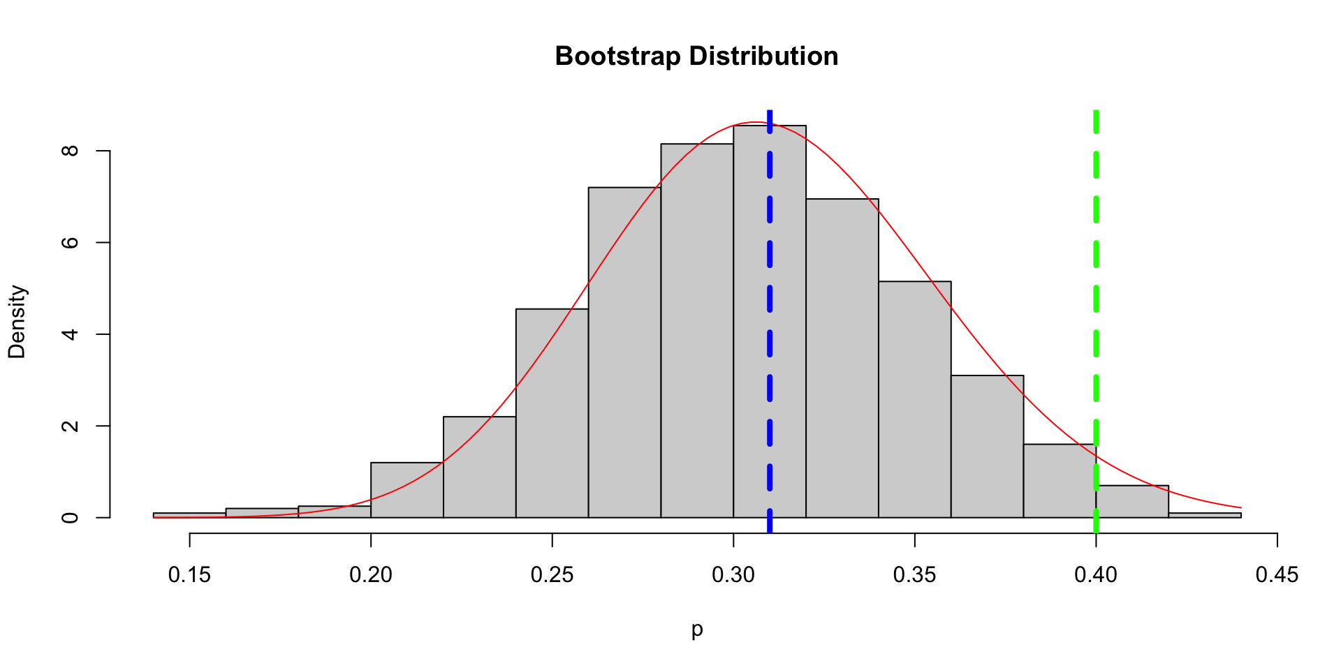
hist(p_boot, freq = FALSE, main = "Bootstrap Distribution", xlab = "p")
curve(dbeta(x, n*p_hat, n*(1-p_hat)), add = T, col = "red")
abline(v = p, lty = 2, col = "green", lwd = 4)
abline(v = p_hat, lty = 2, col = "blue", lwd = 4)Lecture 05: Connections to non-Bayesian Analysis and Hierarchical Models
Chun-Hao Yang
Connections to non-Bayesian Analysis
\[ \newcommand{\mc}[1]{\mathcal{#1}} \newcommand{\R}{\mathbb{R}} \newcommand{\E}{\mathbb{E}} \renewcommand{\P}{\mathbb{P}} \newcommand{\var}{{\rm Var}} % Variance \newcommand{\mse}{{\rm MSE}} % MSE \newcommand{\bias}{{\rm Bias}} % MSE \newcommand{\cov}{{\rm Cov}} % Covariance \newcommand{\iid}{\stackrel{\rm iid}{\sim}} \newcommand{\ind}{\stackrel{\rm ind}{\sim}} \renewcommand{\choose}[2]{\binom{#1}{#2}} % Choose \newcommand{\chooses}[2]{{}_{#1}C_{#2}} % Small choose \newcommand{\cd}{\stackrel{d}{\rightarrow}} \newcommand{\cas}{\stackrel{a.s.}{\rightarrow}} \newcommand{\cp}{\stackrel{p}{\rightarrow}} \newcommand{\bin}{{\rm Bin}} \newcommand{\ber}{{\rm Ber}} \DeclareMathOperator*{\argmax}{argmax} \DeclareMathOperator*{\argmin}{argmin} \]
Introduction
- In the previous lecture, we saw that MLE and MAP are related.
- We will discuss this relationship in more details and explore how this relationship benefits us.
- MLE and MAP are not the only connection between Bayesian and non-Bayesian analysis.
- We will discuss two other examples: bootstrap and random effect model.
MLE vs MAP
- Given \(X_1, \ldots, X_n \iid f(x\mid\theta)\), the likelihood function is
\[\ell(\theta\mid x_1,\ldots,x_n) = \prod_{i=1}^n f(x_i\mid\theta) = f(x_1,\ldots,x_n\mid\theta).\]
- Suppose we choose \(\pi(\theta) \propto 1\). The posterior is1
\[ \pi(\theta \mid x_1, \ldots, x_n) \propto f(x_1,\ldots,x_n\mid\theta)\pi(\theta) = f(x_1,\ldots,x_n\mid\theta). \]
- Therefore
\[ \hat{\theta}_{\text{MAP}} = \argmax_{\theta}\pi(\theta \mid x_1, \ldots, x_n) = \argmax_{\theta}\ell(\theta\mid x_1,\ldots,x_n) = \hat{\theta}_{\text{MLE}}. \]
Asymptotics of MLE
- Let \(X_1, \ldots, X_n \iid f(x\mid \theta)\) and \(\hat{\theta}_n\) be the MLE of \(\theta\).
- Under some regularity conditions on \(f(x\mid\theta)\), the MLE is asymptotically normally distributed and efficient (having the smallest variance).
- That is, \[ \sqrt{n}\left(\hat{\theta}_n-\theta\right) \stackrel{d}{\rightarrow} N\left(0, I(\theta)^{-1}\right) \] where \(I(\theta)\) is the Fisher information of \(f(x\mid\theta)\).
- An important application of this result is the approximate confidence interval for \(\theta\) \[ \P\left(\hat{\theta}_n - z_{\alpha/2}[nI(\hat{\theta}_n)]^{-1/2} \leq \theta \leq \hat{\theta}_n + z_{\alpha/2}[nI(\hat{\theta}_n)]^{-1/2} \right) \approx \alpha. \]
Asymptotics of Bayesian inference
- The Bernstein-von Mises Theorem states that under some regularity conditions, the posterior distribution is asymptotically normal centered at the MLE.
- See Section 10.2 of Van der Vaart (2000) for rigorous arguments.
- The regularity conditions include:
- the posterior must be proper, and
- the prior is (strictly) positive in a neighborhood around the true parameter (this is a strong condition in high dimensions), etc.
- Roughly speaking, the Bernstein-von Mises theorem works well on a problem with few parameters and large dataset containing iid samples. For complicated problems like nonparametric problems, it might not work as well as you expect1.
Normal approximation to the posterior
- If the posterior \(\pi(\theta\mid x)\) is unimodal and roughly symmetric, it can be convenient to approximate it by a normal distribution.
- That is, the logarithm of the posterior density is approximated by a quadratic function of \(\theta\).
- Consider Taylor series expansion of \(\log \pi(\theta\mid x)\) centered at the posterior mode (MAP) \(\hat{\theta}\) \[ \log \pi(\theta \mid x)=\log \pi(\hat{\theta} \mid x)+\frac{1}{2}(\theta-\hat{\theta})^T\left[\frac{d^2}{d \theta^2} \log \pi(\theta \mid x)\right]_{\theta=\hat{\theta}}(\theta-\hat{\theta})+\cdots \]
- That is, \[\begin{align*} \pi(\theta \mid x) \approx N\left(\hat{\theta},[I(\hat{\theta})]^{-1}\right) \end{align*}\] where \(I(\theta)\) is the observed information, \(I(\theta)=-\frac{d^2}{d \theta^2} \log \pi(\theta \mid x)\).
Normal approximation to the posterior
- If the approximation is good, we can construct an approximate credible interval without resorting to sampling techniques.
- In practice, however, it is almost impossible to check how good or bad the approximation is, especially when the parameter is high-dimensional.
- Even for low-dimensional parameter, if the posterior is multi-modal, the normal approximation will be terrible.
- In a later lecture, we will introduce a technique, called variational inference, which allows us to approximate the posterior using any parametric family, not just normal.
Bootstrap and Bayesian Inference1
- Bootstrap is a method proposed by Efron (1979)2 for deriving the sampling distribution of a statistic.
- It is based on resampling from the empirical distribution, which converges to the true population distribution (Glivenko-Cantelli theorem).
- Example: \(X_1, \ldots, X_n \iid F\) and \(\bar{X}_n = \frac{1}{n}\sum_{i=1}^n X_i\).
- A bootstrap sample \(X_1^*, \ldots, X_n^*\) is obtained from \(X_1, \ldots, X_n\) using sampling with replacement.
- The sampling distribution of \(\bar{X}_n\) can be estimated/approximated by the distribution of \(\bar{X}^*_n = \frac{1}{n}\sum_{i=1}^n X_i^*\), which is called the bootstrap distribution.
Bootstrap and Bayesian Inference
- There are some similarities between bootstrap and Bayesian inference:
- They both treat the sample as fixed and given.
- Based on the sample, they both construct a distribution: bootstrap distribution vs posterior distribution.
- When will they be (approximately) the same?
- Suppose \(X_1, \ldots, X_n \mid p \iid \text{Ber}(p)\) and \(p \sim \text{Beta}(\alpha, \beta)\). Then \[ p \sim \text{Beta}\left(\alpha + \sum X_i, \beta + n - \sum X_i\right). \]
- Letting \(\alpha \to 0\) and \(\beta \to 0\), we have a noninformative prior and \[ p \mid X_1,\ldots, X_n \sim \text{Beta}\left(\sum X_i, n-\sum X_i\right). \]
Bootstrap and Bayesian Inference
- Consider a bootstrap sample \(X_1^*, \ldots, X_n^*\) (obtained from \(X_1,\ldots,X_n\) using sampling with replacement).
- Actually, \(X_1^*,\ldots, X_n^*\mid X_1,\ldots, X_n \iid \text{Ber}(\hat{p})\), where \(\hat{p} = \frac{1}{n}\sum X_i\).
- Let \(\hat{p}^* = \frac{1}{n}\sum X_i^*\). What is the bootstrap distribution \(\hat{p}^* \mid X_1,\ldots, X_n\)?
- Let’s do some experiment!
Bootstrap and Bayesian Inference
Bootstrap and Bayesian Inference
Bootstrap and Bayesian Inference
- In this sense, the bootstrap distribution represents an (approximate) nonparametric posterior distribution under a noninformative prior.
- But this bootstrap distribution is obtained painlessly – without having to formally specify a prior and without having to sample from the posterior distribution.
- Hence we might think of the bootstrap distribution as a “poor man’s” posterior.
Distributional estimates
- One of the advantages of Bayesian inference is that the entire inference is based the posterior distribution, rather than a single point estimate or an interval.
- The posterior distribution is just one example of distributional estimate, which use a distribution for inference.
- Bootstrap distribution is another example.
- There is a frequentist concept, called the confidence distribution, proposed by Neyman (1937)1.
- The confidence distribution contains confidence interval of any level.
- Fraser (2011)2 also discussed how the Bayesian posterior and the confidence distribution are related.
Random effect models
- Fixed effect model: \(Y_i = \beta_0 + \beta X_i + \varepsilon_i\), \(\varepsilon_i \iid N(0, \sigma^2)\)
- The parameter \(\beta\) is the fixed effect of the factors \(X\).
- With a unit increase in \(X\), \(Y\) is expected to increase by \(\beta\).
- Use (regularized) least squares to obtain an estimate for \(\beta\).
- The effect is the same for each observation
- Random effect model: \(Y_i = \beta_0 + \gamma_iX_i + \varepsilon_i\), \(\gamma_i \sim N(\beta, \tau^2)\), \(\varepsilon_i \iid N(0, \sigma^2)\)
- \(\gamma_i\) is the random effect in this model
- The effect is different for each observation and, on average, \(Y\) is increase by \(\beta\) with a unit increase in \(X\).
Mixed effect model
- A model with both fixed effects and random effects is called a mixed effect model.
- This model is commonly used in biostatistics, psychology, economics, etc.
- A typical mixed effect model: \[ Y = X\beta + Z\gamma + \varepsilon, \quad \varepsilon \sim N(0, \sigma^2) \] where \(\beta\) is the unknown fixed effect and \(\gamma \sim N(\nu, \Psi)\) is the unknown random effect.
Sleep deprivation study
Data description
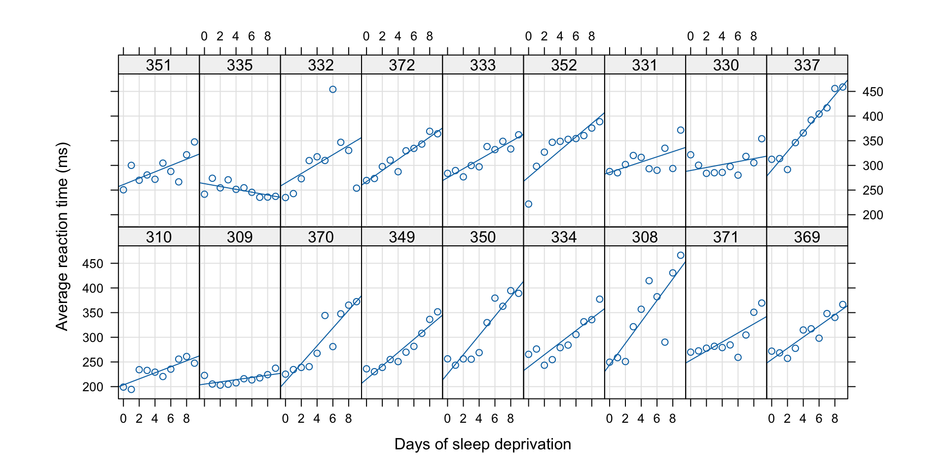
We use the sleepstudy dataset in the lme4 R package.
This dataset contains the average reaction time per day (in milliseconds) for subjects in a sleep deprivation study described in Belenky et al. (2003)1, for the most sleep-deprived group (3 hours time-in-bed; 18 subjects) and for the first 10 days of the study. Days 0-1 were adaptation and training (T1/T2), and day 2 was baseline (B); sleep deprivation started after day 2.
Data description
First attempt: simple linear regression
- Let \(Y\) be the reaction time and \(X\) be the Day variable.
- We want to see the negative impact of consecutive sleep loss in reaction time.
- A simple linear model: \(Y = \beta_0 + \beta_1 X\).
Individual difference
However, this model does not take into account the individual difference, i.e., the difference between subjects.
Second attempt: Mixed effect model
- We allow each subject to have its own intercept and effect: \[ Y_{ij} = b_{0,i} + b_{1,i} X_{j}, \quad i = 1,\ldots, 18, j = 0,\ldots, 9 \] where \(Y_{ij}\) is the reaction time of \(i\)th subject in Day \(j\).
- Note that we are not interested in the effects for each individuals.
- We just want to identify how much the individual difference contributes to the un-explained variation of the model.
- We assume that \(b_{0,i} \iid N(\beta_0, \tau_0^2)\) and \(b_{1,i} \iid N(\beta_1, \tau_1^2)\) are independent.
- The frequentist interpretation of this assumption is that the subjects are randomly selected, so there is randomness in the individual coefficients.
- The parameters \(\beta_0\) and \(\beta_1\) are unknown and fixed.
Second attempt: Mixed effect model
sleepstudy |>
    lmer(Reaction ~ Days + (1|Subject) + (0+Days|Subject),
         data = _, subset=Days>=2) |>
tab_model(show.icc = FALSE,show.obs = FALSE, show.ngroups = FALSE)| Reaction | |||
|---|---|---|---|
| Predictors | Estimates | CI | p |
| (Intercept) | 245.10 | 227.71 – 262.49 | <0.001 |
| Days | 11.44 | 7.97 – 14.90 | <0.001 |
| Random Effects | |||
| σ2 | 662.92 | ||
| τ00 Subject | 831.93 | ||
| τ11 Subject.Days | 39.50 | ||
| ρ01 | |||
| ρ01 | |||
| Marginal R2 / Conditional R2 | 0.316 / 0.697 | ||
Bayesian approach to mixed effect models
- The random effect assumption looks like a prior distribution on the coefficients.
- A mixed model \[ Y = X\beta + Z\gamma + \varepsilon, \quad\gamma \sim N(\nu, \Psi), \varepsilon \sim N(0, \sigma^2) \] can be rewritten as \[\begin{align*} Y \mid \gamma & \sim N(X\beta + Z\gamma, \sigma^2)\\ \gamma & \sim N(\nu, \Psi) \end{align*}\]
- A Bayesian approach puts priors on the parameters: \[\begin{align*} Y \mid \gamma, \beta, \sigma^2 & \sim N(X\beta + Z\gamma, \sigma^2)\\ \gamma \mid \nu, \Psi & \sim N(\nu, \Psi)\\ \beta, \nu, \sigma^2, \Psi & \sim \pi(\beta, \nu, \sigma^2, \Psi) \end{align*}\]
Bayesian approach to mixed effect models
Use stan_lmer to fit a Bayesian mixed effect model
- Use
summary(sleep_lmer_B)to check the fitted result - Use
prior_summary(sleep_lmer_B)to check the priors used in the model
Wrap-up
- Random effects are also called variance components, since we are more interested in the variance of the random effect rather than the effect itself.
- Mixed effect model is just one example of hierarchical models (or multi-level models).
- A hierarchical model contains many sub-models that are linked by some hierarchical relations.
- In the previous example, we can partition the dataset into smaller pieces by subject and hence subject is a hierarchy in this dataset.
- Note that a hierarchical model need not be a Bayesian model. However, Bayesian approach is a natural way to fit a hierarchical model.
Hierarchical Models
Motivation
- Some problems have intrinsic hierarchical structures, e.g., samples are grouped by some covariates (gender, ethnicity, etc.).
- In practice, simple nonhierarchical models are usually inappropriate for hierarchical data: with few parameters, they generally cannot fit large datasets accurately, whereas with many parameters, they tend to ‘overfit’.
- When parameters are only exchangeable rather than independent, a hyperprior is needed (de Finetti’s Theorem). That is, the subscripts of the parameters convey no information.
Meta-analysis
Meta-analysis is an increasingly popular and important process of summarizing and integrating the findings of research studies in a particular area.
The article “Why Science Is Not Necessarily Self-Correcting” by Ioannidis (2012) pointed out that sometimes fundamental fallacies remain unchallenged and are only perpetuated.
You can find a detailed introduction to meat-analysis and different approaches to meta-analysis in https://bookdown.org/MathiasHarrer/Doing_Meta_Analysis_in_R/.
Clinical trials of beta-blockers
Data description
- Beta-blocker is a family of drugs that affect the central nervous system and can relax the heart muscles.
- This dataset summarizes mortality after myocardial infarction in 22 clinical trials.
- Each clinical trial consists of two groups of heart attack patients randomly allocated to receive or not receive beta-blockers.
- The dataset is available at http://www.stat.columbia.edu/~gelman/book/data/meta.asc.
- The aim of a meta-analysis is to provide a combined analysis of the studies that indicates the overall strength of the evidence for a beneficial effect of the treatment under study.
Data description
Odds ratio
- The odds ratio is the ratio of the odds death in the treatment group and the odds of death in the control group \[ \rho = \left. \frac{p_{\text{treat}}}{1-p_{\text{treat}}} \middle/ \frac{p_{\text{con}}}{1-p_{\text{con}}} \right. . \]
- We concentrate the inference on the log of the odds ratios \(\theta = \log \rho\) for each clinical trial.
Normal approximation to the likelihood
- Let \(y_{ij}\) and \(n_{ij}\) be the number of deaths and subjects of the \(i\)th group (\(1=\) treated, \(0 =\) control) in study \(j\).
- For each study \(j\), we estimate \(\theta_j\) by \[ \hat{\theta}_j=\log \left(\frac{y_{1 j}}{n_{1 j}-y_{1 j}}\right)-\log \left(\frac{y_{0 j}}{n_{0 j}-y_{0 j}}\right), \] with approximate sampling variance \[ \sigma_j^2=\frac{1}{y_{1 j}}+\frac{1}{n_{1 j}-y_{1 j}}+\frac{1}{y_{0 j}}+\frac{1}{n_{0 j}-y_{0 j}}. \]
- Thus \(\hat{\theta}_j \sim N(\theta_j, \sigma_j^2)\) approximately.
Odds ratio
meta_summary <- meta |>
    mutate(treated.odds = treated.deaths/(treated.total - treated.deaths),
           control.odds = control.deaths/(control.total - control.deaths),
           log.odds.ratio = log(treated.odds) - log(control.odds),
           var = 1/treated.deaths + 1/(treated.total - treated.deaths) +
               1/control.deaths + 1/(control.total - control.deaths)) |>
    select(c(study, log.odds.ratio, var))
meta_summary |> head() |> kbl(digits = 4)| study | log.odds.ratio | var |
|---|---|---|
| 1 | 0.0282 | 0.7230 |
| 2 | -0.7410 | 0.2334 |
| 3 | -0.5406 | 0.3187 |
| 4 | -0.2461 | 0.0191 |
| 5 | 0.0695 | 0.0788 |
| 6 | -0.5842 | 0.4566 |
Goal of the inference
- Now we have the log odds ratios and their sampling variances from 22 studies.
- How are these studies related to each other?
- Are they identical replications of each other, i.e., the studies are independent samples from a common population?
- Are they completely unrelated?
- A more realistic assumption is that they are somewhere between the two extremes.
- Exchangeablity assumption: the parameters \(\theta_j\) are exchangeable.
- We cannot distinguish \(\theta_j\)’s before we see that data.
- Therefore \[ (\theta_1, \ldots, \theta_{22}) \sim \pi \Leftrightarrow \theta_i \iid \pi(\theta\mid\phi), \phi \sim \nu. \]
A hierarchical model
- Likelihood: \(\hat{\theta}_j \sim N(\theta_j, \sigma^2_j)\), \(j = 1,\ldots, 22\).
- Assume the \(\sigma^2_j\)’s are known (given by the sampling variance computed before).
- Prior: we use the exchangeable normal prior for \(\theta_j\), \[ \theta_j \mid \mu, \tau \iid N(\mu, \tau^2) \] where \(\mu\) and \(\tau\) are unknown hyperparameters.
- Hyperprior: for \(\mu\) and \(\tau\) \[\begin{align*} \mu & \sim \pi(\mu) \propto 1\\ \tau & \sim \text{Unif}(0, A) \end{align*}\] for some large \(A\).
- Computation is left as homework.
Weakly informative priors for variance parameters
- For the variance parameter \(\tau\), we use the uniform prior \(\text{Unif}(0, A)\), which is a proper noninformative prior.
- Another choice is Inverse-Gamma\((\epsilon, \epsilon)\), with small \(\epsilon\).
- How about the Jeffreys prior?
- To compute the Jeffreys prior, you need to first find the marginal distribution \(f(x\mid \mu, \tau) = \int f(x \mid \theta) \pi(\theta \mid \mu, \tau) d\theta\).
- Then compute the Fisher information of \(f(x \mid \mu, \tau)\).
- Both steps are difficult!!
- A bad news is that the posterior of \(\tau\) is sensitive to the choice of prior. You will see this in your homework.
- Read Section 5.7 of BDA for more details.