set.seed(2023)
m <- 10000
x <- c()
for(i in 1:m){
    v <- runif(1) # proposal

    # rejection step
    u <- runif(1)
    if(u <= dbeta(v, alpha, beta) / (3 * dunif(v))){
        x <- c(x, v)
    }
}

hist(x, freq = FALSE, xlim = c(0,1))
curve(dbeta(x, alpha, beta), col = "red", lwd = 2, add = TRUE)
text(0.1, 2, substitute("accept. rate" == a,
list(a = round(length(x)/m, 2))))Lecture 07: Markov Chain Monte Carlo
Chun-Hao Yang
Motivation
\[ \newcommand{\mc}[1]{\mathcal{#1}} \newcommand{\R}{\mathbb{R}} \newcommand{\E}{\mathbb{E}} \renewcommand{\P}{\mathbb{P}} \newcommand{\var}{{\rm Var}} % Variance \newcommand{\mse}{{\rm MSE}} % MSE \newcommand{\bias}{{\rm Bias}} % MSE \newcommand{\cov}{{\rm Cov}} % Covariance \newcommand{\iid}{\stackrel{\rm iid}{\sim}} \newcommand{\ind}{\stackrel{\rm ind}{\sim}} \renewcommand{\choose}[2]{\binom{#1}{#2}} % Choose \newcommand{\chooses}[2]{{}_{#1}C_{#2}} % Small choose \newcommand{\cd}{\stackrel{d}{\rightarrow}} \newcommand{\cas}{\stackrel{a.s.}{\rightarrow}} \newcommand{\cp}{\stackrel{p}{\rightarrow}} \newcommand{\bin}{{\rm Bin}} \newcommand{\ber}{{\rm Ber}} \DeclareMathOperator*{\argmax}{argmax} \DeclareMathOperator*{\argmin}{argmin} \]
- Suppose now we have the posterior distribution \(\pi(\theta \mid x)\) for our problem.
- We need to derive some quantities from the posterior for statistical inference, for example
- posterior mean, variance, quantiles, and
- posterior predictive distribution.
- We have seen that in many cases, the posterior is only available upto a normalizing constant.
- There are three types of methods:
- numerical integration,
- distributional approximations, and
- sampling-based methods (Monte Carlo methods).
Monte Carlo Methods
Suppose we need to compute \(\E(h(\theta) \mid x)\).
The Monte Carlo approximation is \[ \E(h(\theta) \mid x) \approx \frac{1}{m}\sum_{i=1}^m h(\theta^{(i)}), \] where \(\theta^{(1)}, \ldots, \theta^{(m)} \iid \pi(\theta \mid x)\).
How to generate iid random samples from an arbitrary distribution?
How to do it without knowing the normalizing constant?
Discretization
- Fix a set of grid values \(\theta_1, \ldots, \theta_N\).
- Compute \(\pi(\theta_1 \mid x), \ldots \pi(\theta_N \mid x)\) and normalize them such that \[ \sum_{i=1}^N \pi(\theta_i \mid x) = 1. \]
- Generate \(m\) samples from the multinomial distribution with probabilities \(\pi(\theta_1 \mid x), \ldots, \pi(\theta_N \mid x)\).
- That is, we approximate \(\pi(\theta \mid x)\) on \(\Theta\) with a multinomial distribution on \(\{\theta_1, \ldots, \theta_N\}\).
Rejection sampling
- Target distribution: \(\pi(\theta \mid x)\) (possibly unnormalized)
- We need a proposal distribution \(q(\theta)\) such that
- it is easy to sample from \(q(\theta)\), and
- the importance ratio \(\pi(\theta \mid x) / q(\theta)\) is bounded, i.e., \[ \frac{\pi(\theta \mid x)}{q(\theta)} \leq M < \infty, \quad \text{for all } \theta \in \Theta. \]
- Algorithm:
- Sample \(\theta \sim q(\theta)\).
- With probability \(\frac{\pi(\theta \mid x)}{M q(\theta)}\), accept \(\theta\) as a draw from \(\pi(\theta \mid x)\). If the drawn \(\theta\) is rejected, return to step 1.
- Repeat steps 1 and 2 until \(m\) samples are obtained.
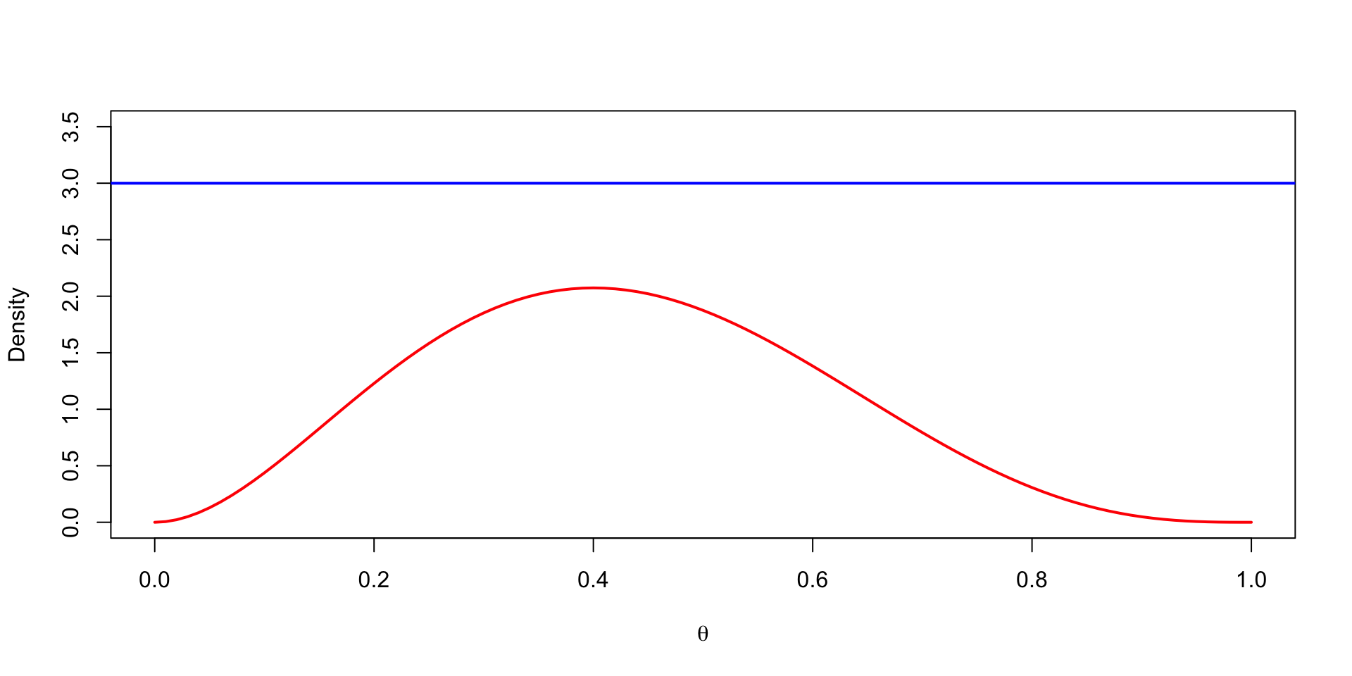
Example
Generate random samples from \(\text{Beta}(\alpha, \beta)\), \(\alpha = 3\) and \(\beta = 4\).
- Proposal distribution: \(\text{Unif}(0, 1)\).
- \(M = 3\).
Example
Example

Problems with rejection sampling
- If \(M\) is large, then the acceptance rate is low, and hence the algorithm is inefficient.
- You have to know \(\pi(\theta \mid x)\) well to find a good proposal distribution, with a reasonable \(M\).
- For multivariate distributions, it is virtually impossible to find a good proposal distribution.
- However, it can be used for simple univariate distributions or truncated distributions.
- Although rejection sampling produces iid samples from the target distribution, it is inefficient.
Markov Chain Monte Carlo
Markov Chain Monte Carlo (MCMC)
- MCMC uses samples from a Markov chain whose stationary distribution is the target distribution.
- Hence the samples are not independent and not from the target distribution.
- They are only iid from the target distribution asymptotically.
- The problem is now how to construct a Markov chain whose stationary distribution is the posterior.
- We will introduce three algorithms:
- Gibbs sampler
- Metropolis-Hastings algorithm
- Hamiltonian Monte Carlo (HMC)
Gibbs Sampler
- Consider a parameter vector \(\theta = (\theta_1, \theta_2, \ldots, \theta_p)\) with posterior \(\pi(\theta|y)\).
- If we can sample from the full conditional distributions \(\pi(\theta_i|\theta_{-i}, y)\), then we can construct a Markov chain whose stationary distribution is the posterior.
- Algorithm:
- Initialize \(\theta^{(0)} = (\theta_1^{(0)}, \theta_2^{(0)}, \ldots, \theta_p^{(0)})\).
- For \(t = 1, 2, \ldots, T\):
- Sample \(\theta_1^{(t)} \sim \pi(\theta_1|\theta_2^{(t-1)}, \theta_3^{(t-1)}, \ldots, \theta_p^{(t-1)}, y)\).
- Sample \(\theta_j^{(t)} \sim \pi(\theta_2|\theta_1^{(t)}, \ldots, \theta_{j-1}^{(t)}, \theta_{j+1}^{(t-1)}, \ldots, \theta_p^{(t-1)}, y)\).
- Return \(\theta^{(1)}, \theta^{(2)}, \ldots, \theta^{(T)}\).
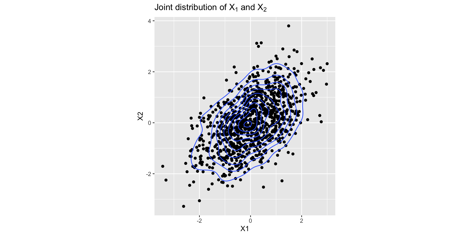
Example: Bivariate Normal
- Suppose we want to generate samples from a bivariate normal with mean \(\mu = (\mu_1, \mu_2)\) and covariance matrix \(\Sigma\).
- Let \([X_1, X_2]^T \sim N(\mu, \Sigma)\). The full conditionals are:
- \(X_1|X_2 \sim N(\mu_1 + \Sigma_{12}\Sigma_{22}^{-1}(X_2 - \mu_2), \Sigma_{11} - \Sigma_{12}\Sigma_{22}^{-1}\Sigma_{21})\).
- \(X_2|X_1 \sim N(\mu_2 + \Sigma_{21}\Sigma_{11}^{-1}(X_1 - \mu_1), \Sigma_{22} - \Sigma_{21}\Sigma_{11}^{-1}\Sigma_{12})\).
# initialize
mu <- c(0, 0)
Sigma <- matrix(c(1, 0.5, 0.5, 1), nrow = 2)
X <- matrix(0, nrow = 2, ncol = 1000)

# Gibbs sampler
for (t in 2:1000) {
    X[1, t] <- rnorm(1, mu[1] + Sigma[1, 2] / Sigma[2, 2] * (X[2, t-1] - mu[2]),
                     sqrt(Sigma[1, 1] - Sigma[1, 2] / Sigma[2, 2] * Sigma[2, 1]))
    X[2, t] <- rnorm(1, mu[2] + Sigma[2, 1] / Sigma[1, 1] * (X[1, t] - mu[1]),
                     sqrt(Sigma[2, 2] - Sigma[2, 1] / Sigma[1, 1] * Sigma[1, 2]))
}
Checking Convergence
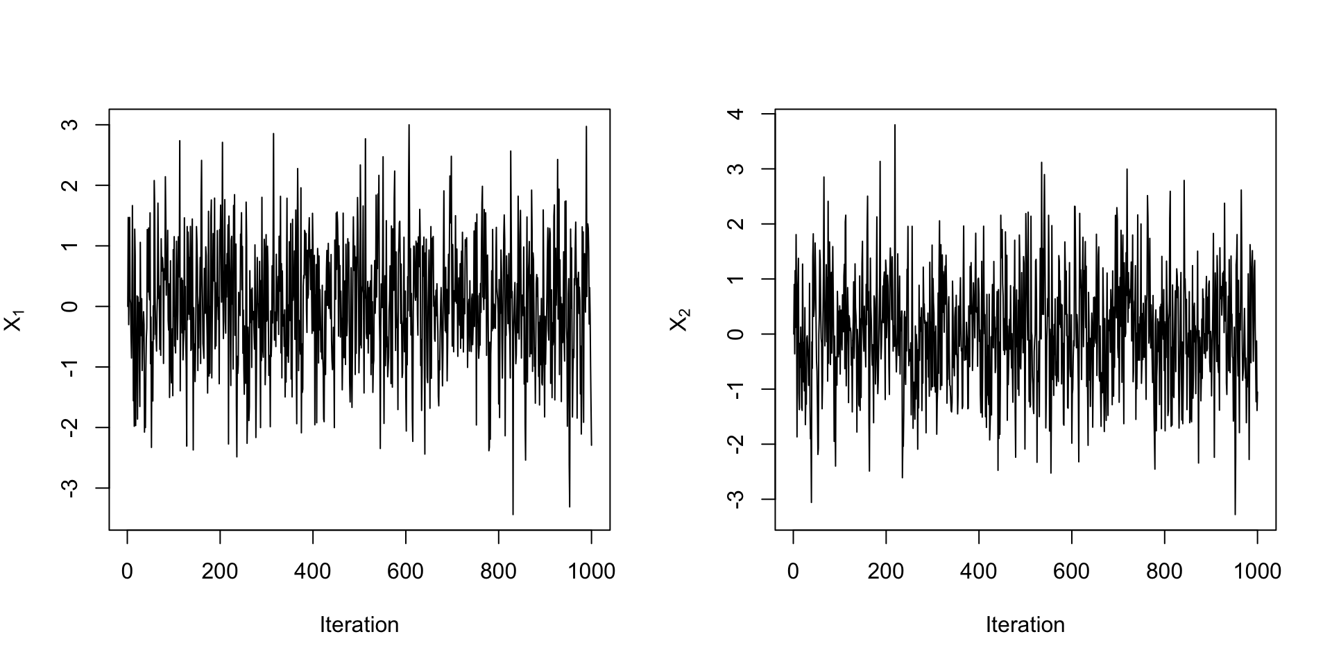
Checking Convergence
When to use Gibbs sampler?
- It is useful for multidimensional distributions, especially when the full conditionals are easy to sample from.
- Even if the full conditionals are not easy to sample from, we can use other algorithms to sample from the conditionals.
Metropolis Algorithm
- Target distribution: \(\pi(\theta \mid x)\).
- Proposal distribution at \(t\)th iteration: \(J_t(\theta^* \mid \theta^{(t-1)})\)
- \(J_t\) needs to be symmetric, i.e., \(J_t(\theta_1 \mid \theta_2) = J_t(\theta_2\mid\theta_1)\).
- Algorithm:
- At \(t\)th iteration, sample \(\theta^*\) from \(J_t(\theta^* \mid \theta^{(t-1)})\).
- Compute the acceptance ratio \(\rho(\theta^{(t-1)}, \theta^{*})=\min\left\{\frac{\pi(\theta^* \mid x)}{\pi(\theta^{(t-1)} \mid x)}, 1\right\}\).
- Set \[ \theta^{(t)}= \begin{cases}\theta^* & \text { with prob. } \rho(\theta^{t-1}, \theta^{*}) \\ \theta^{(t-1)} & \text { with prob. } 1-\rho(\theta^{(t-1)}, \theta^{*}).\end{cases} \]
- Intuition: if \(\theta^*\) is more likely than \(\theta^{(t-1)}\), then accept \(\theta^*\); otherwise, accept \(\theta^*\) with probability \(\rho(\theta^{(t-1)}, \theta^{*})\).
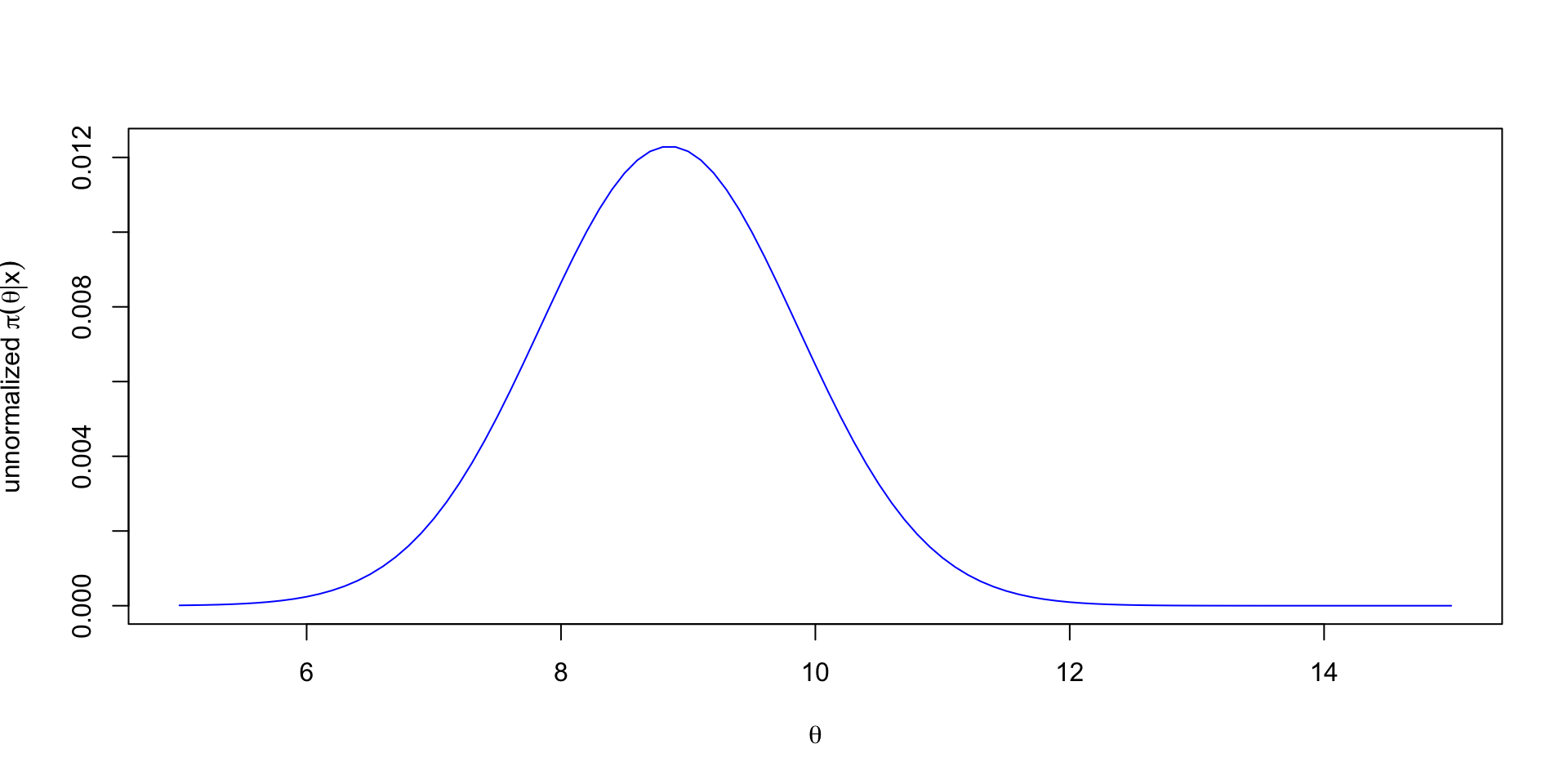
Example
- Suppose \(X \mid \theta \sim N(\theta, 1)\) and \(\theta \sim \text{Cauchy}(0, 1)\).
- The posterior is \(\pi(\theta \mid x) \propto \frac{1}{1+\theta^2}\exp\left(-\frac{1}{2}(x-\theta)^2\right)\).
- A commonly used proposal is \(J_t(\cdot \mid\theta^{(t-1)}) = N(\theta^{(t-1)}, \sigma^2)\), where \(\sigma^2\) is a tuning parameter.
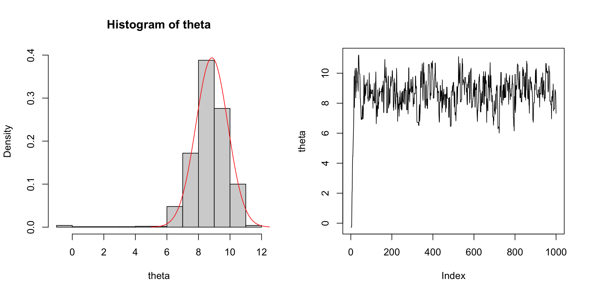
Example
Example
- Acceptance rate: 0.702.
- Autocorrelation (lag 1): 0.823, i.e., the correlation between \(\theta^{(t-1)}\) and \(\theta^{(t)}\).
- Posterior mean: 8.635.
Example
Advantages of Metropolis Algorithm
- It can be seen as a improvement of rejection sampling.
- We don’t need to know the target distribution well to choose a proposal distribution.
- The trade-off is that the generated samples are not longer iid.
- We can tune the proposal distribution to improve the acceptance rate making the algorithm more efficient.
Metropolis-Hastings Algorithm
- Metropolis-Hastings algorithm is a generalization of Metropolis algorithm, in that it does not require symmetric proposals.
- For a proposal distribution \(J_t(\theta_a \mid \theta_b)\), the unconditional probability from \(\theta_a\) to \(\theta_b\) is \[ p(\theta^{t-1} = \theta_a, \theta^{t} = \theta_b) = J_t(\theta_b \mid \theta_a)\pi(\theta_a \mid x). \]
- Hence the acceptance ratio becomes \[\begin{align*} \rho(\theta^{t-1}, \theta^{*}) & = \min\left\{\frac{p(\theta^{t-1} = \theta^{t-1}, \theta^{t} = \theta^{*})}{p(\theta^{t-1} = \theta^{*}, \theta^{t} = \theta^{t-1})},1\right\}\\ & = \min\left\{\frac{J_t(\theta^{t-1} \mid \theta^{*})\pi(\theta^{*} \mid x)}{J_t(\theta^{*} \mid \theta^{t-1})\pi(\theta^{t-1} \mid x)},1\right\}. \end{align*}\]
- This modification allows us to use a wider range of proposal distributions and hence improve the efficiency of the algorithm.
Why it works?
- It is obvious that MH generates a Markov chain. Why does it converge to the target distribution?
- Detailed balance condition1: A Markov chain has a stationary distribution \(\pi\) if it satisfies the equation \[ \pi(\theta_a)\P(X_t = \theta_b \mid X_{t-1} = \theta_a) = \pi(\theta_b)\P(X_t = \theta_a \mid X_{t-1} = \theta_b). \]
- Proof (sketch): \[\begin{align*} & \quad \pi(\theta_a \mid x)\P(X_t = \theta_b \mid X_{t-1} = \theta_a)\\ &= \pi(\theta_a \mid x)J_t(\theta_b \mid \theta_a) \rho(\theta_a, \theta_b) \\ & = \pi(\theta_a \mid x)J_t(\theta_b \mid \theta_a) \min\left\{\frac{J_t(\theta_a \mid \theta_b)\pi(\theta_b \mid x)}{J_t(\theta_b \mid \theta_a)\pi(\theta_a \mid x)},1\right\}\\ & = \min\left\{J_t(\theta_a \mid \theta_b)\pi(\theta_b \mid x), J_t(\theta_b \mid \theta_a)\pi(\theta_a \mid x)\right\} \end{align*}\]
Ergodic Theorems
- Now we know that the MH algorithm generates a Markov chain \(\theta_1, \theta_2, \ldots\) with a stationary distribution \(\pi(\theta \mid x)\).
- We need to use these MCMC samples to estimate posterior quantities, for example, \[ \frac{1}{M}\sum_{i=1}^M h(\theta_i). \]
- If the \(\theta_i\)’s are iid, then we can use the CLT to obtain the consistency and the asymptotic distribution of the above estimator.
- For Markov chains, we have ergodic theorems, which state that if \(\theta_1,\theta_2,\ldots\) is ergodic, we have the CLT.
- See Ch. 6 & 7 of Monte Carlo Statistical Methods by Robert & Casella (2004) for details.
Guidelines for choosing proposal distribution
- For any \(\theta\), it is easy to sample from \(J\left(\theta^* \mid \theta\right)\).
- It is easy to compute the ratio \(\rho\).
- Each jump goes a reasonable distance in the parameter space (otherwise the random walk moves too slowly).
- The jumps are not rejected too frequently (otherwise the random walk wastes too much time standing still).
Combining Gibbs and MH
- In fact, Gibbs sampler is a special case of MH, with the proposal being the conditional distribution: \[ J_{j, t}^{\text {Gibbs }}\left(\theta^* \mid \theta^{(t-1)}\right)= \begin{cases}\pi\left(\theta_j^* \mid \theta_{-j}^{(t-1)}, x\right) & \text { if } \theta_{-j}^*=\theta_{-j}^{(t-1)} \\ 0 & \text { otherwise. }\end{cases} \]
- We can use MH to sample from \(\pi\left(\theta_j^* \mid \theta_{-j}^{(t-1)}, x\right)\). This is called Metropolis-within-Gibbs.
- In cases where some conditionals are easy to sample from but others are not, Metropolis-within-Gibbs will be more efficient than a simple MH.
Diagnostic of MCMC
Diagnostic of MCMC samples
Suppose now we have a sequence of MCMC samples: \(\theta_1, \ldots, \theta_m\).
- Did I run the chain long enough so that the samples are roughly from the target distribution?
- How strong is the dependence between the samples?
- How to fix these problems?
Mixing and convergence
- Convergence: whether the chain has converged to the target distribution.
- Mixing: Multiple chains should mix together.
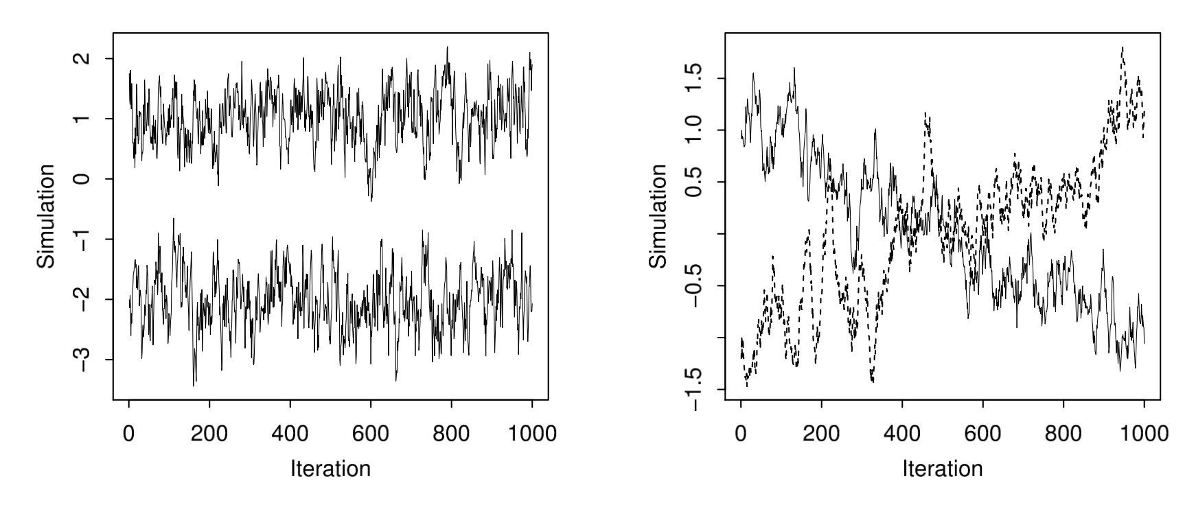
Fig 11.3 of BDA
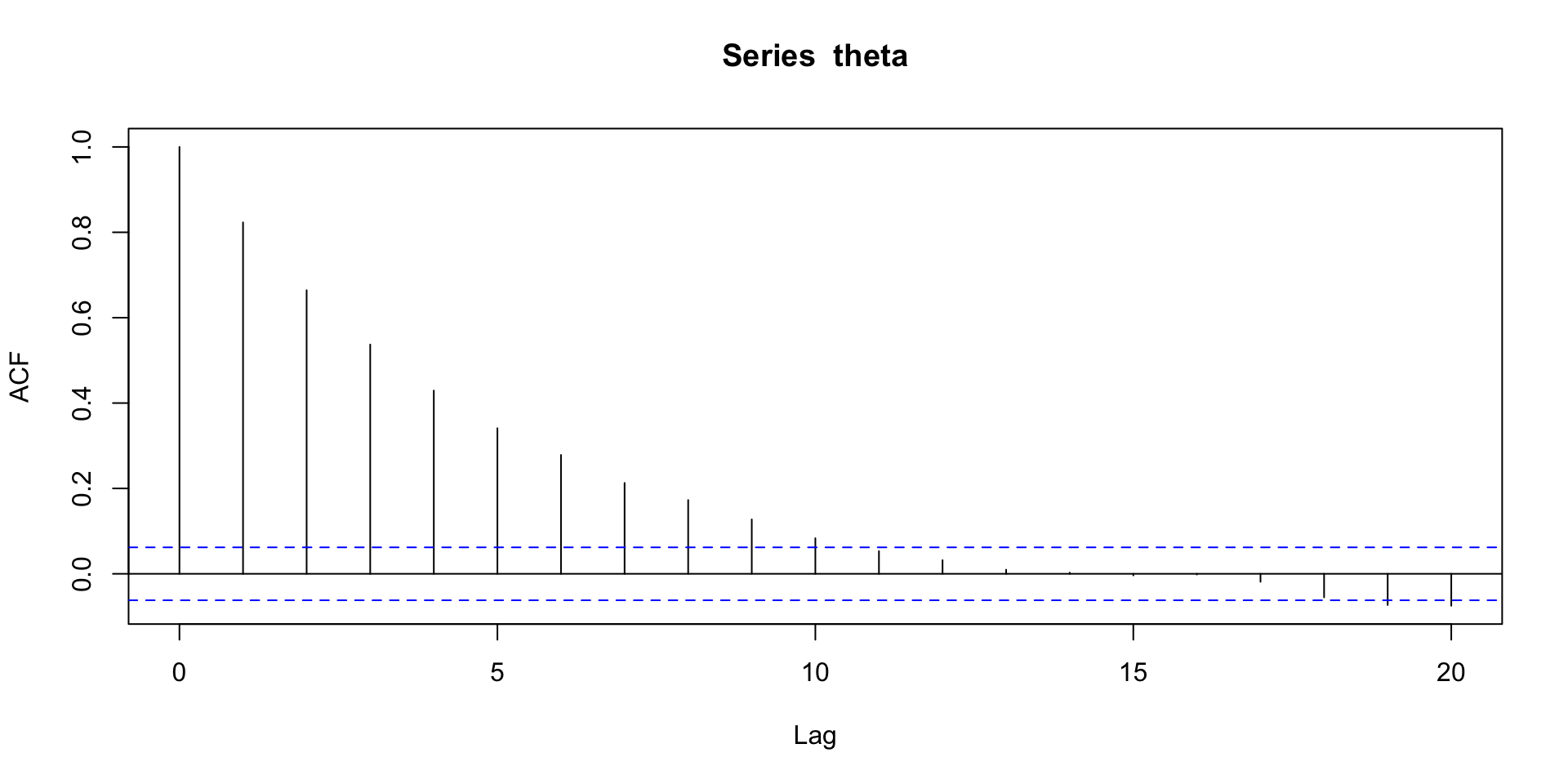
Autocorrelation
Lag-\(k\) Autocorrelation: the correlation between \(\theta^{(t)}\) and \(\theta^{(t+k)}\) for \(k > 0\).
Effective sample size
- We can compute an approximate ``effective number of independent simulation draws’’ for any estimand of interest \(\psi\).
- The effective sample size is defined as \[ \text{ESS} = \frac{m}{1 + 2\sum_{k=1}^\infty \rho_k}, \] where \(m\) is the length of a chain and \(\rho_k\) is the lag-\(k\) autocorrelation.
- Different estimates of \(\rho_k\)’s give different ESS’s.
Practical tricks
- Burn-in: discard the first few samples.
- Thinning: keep only every \(k\)-th sample.
- Simulated annealing: start with a large variance (of proposal) and gradually reduce it.
- Parallel tempering: run multiple chains with different temperatures and swap chains occasionally: for \(1 < T_1 < T_2 < \cdots < T_n\), the \(i\)-th chain has target distribution \[ \pi_i(\theta) \propto \pi(\theta)^{1/T_i} = \exp\left\{\frac{1}{T_i}\log\pi(\theta)\right\}. \]
- Data augmentation: introduce latent variables to make the target distribution more tractable, i.e., find \(\nu\) such that \[ \pi(\theta \mid x) = \int \pi(\theta \mid \xi, x) \nu(\xi)d\xi. \]
Example
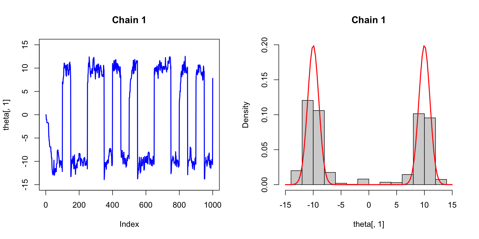
Suppose the target distribution is \(\pi(\theta) = \frac{1}{2}N(10,1) + \frac{1}{2}N(-10, 1)\).
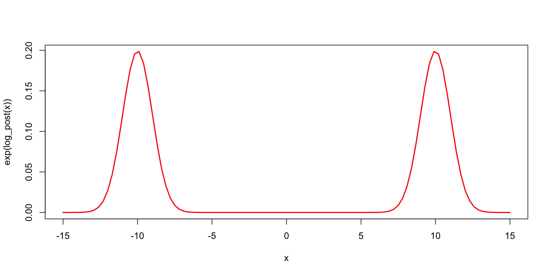
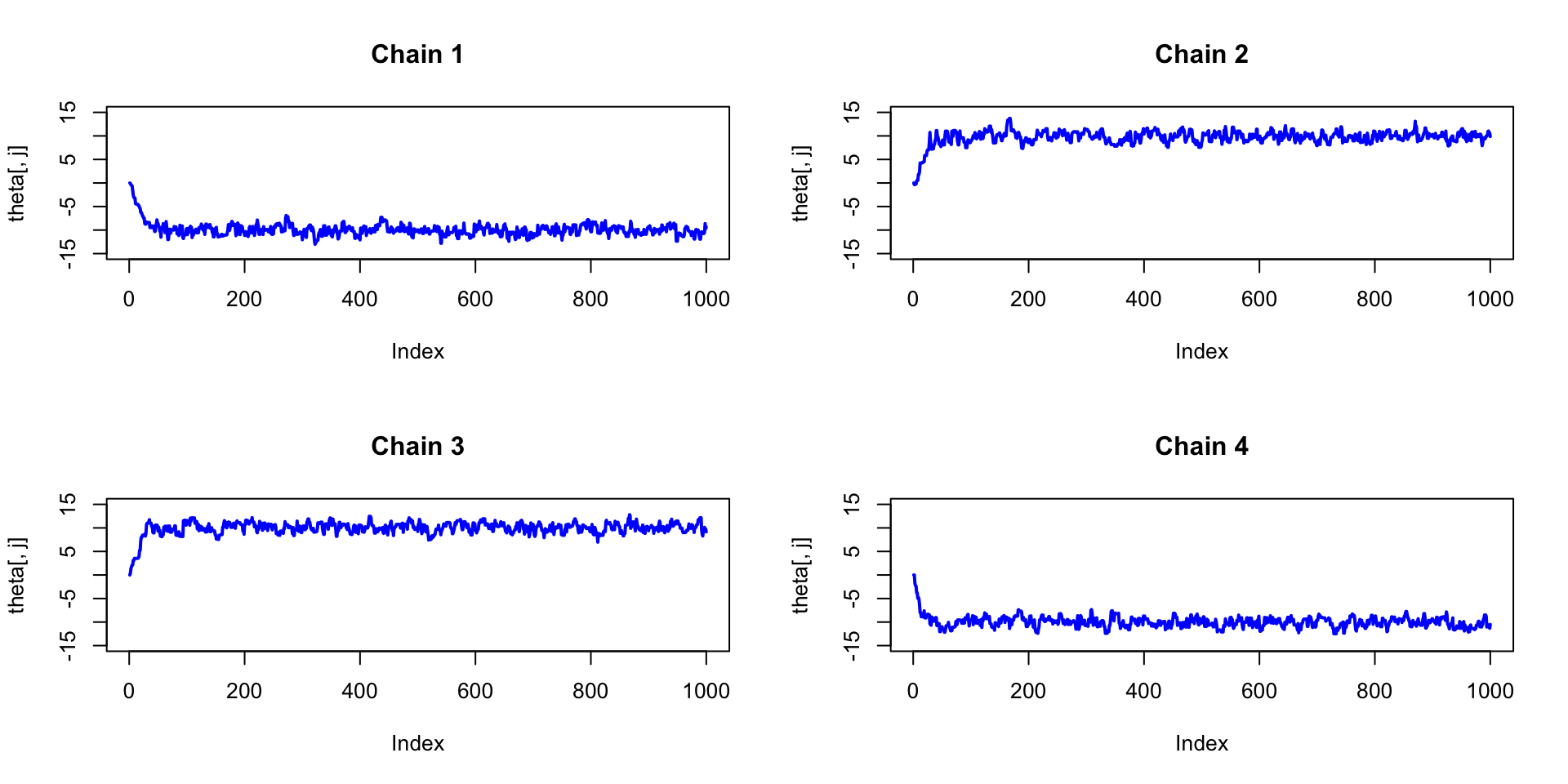
Vanilla Metropolis
set.seed(2023)
M <- 1000; n_chain <- 4
theta <- matrix(0, ncol = 4, nrow = M)

for (j in 1:n_chain){
    for (i in 2:M){
        theta.star <- rnorm(1, theta[i-1,j], 1)
        rho <- exp(log_post(theta.star) - log_post(theta[i-1,j]))
        if (runif(1) < rho){
            theta[i,j] <- theta.star
        } else {
            theta[i,j] <- theta[i-1,j]
        }
    }
}
Vanilla Metropolis
Parallel tempering
set.seed(2023)
M <- 1000; n_chain <- 4
theta <- matrix(0, ncol = 4, nrow = M)
temp <- c(1, 10, 20, 40); swap_int <- 50

for (i in 2:M){
    for (j in 1:n_chain){
        theta.star <- rnorm(1, theta[i-1,j], 1)
        rho <- exp(log_post(theta.star)/temp[j] -
                       log_post(theta[i-1,j])/temp[j])
        if (runif(1) < rho){
            theta[i,j] <- theta.star
        } else {
            theta[i,j] <- theta[i-1,j]
        }
    }
    # Swap chains
    if(i %% swap_int == 0){
        for (j in 1:(n_chain-1)){
            rho <- exp(log_post(theta[i,j])/temp[j+1] +
                           log_post(theta[i,j+1])/temp[j] -
                           log_post(theta[i,j])/temp[j]-
                           log_post(theta[i,j+1])/temp[j+1])
            if (runif(1) < rho){
                theta[i,] <- theta[i, c(j+1, j)]
            }
        }
    }
}
Parallel tempering