Lecture 09: Bayesian Regression

Chun-Hao Yang

Classical Linear regression

Linear regression

Suppose we have samples \(\{x_i, y_i\}_{i=1}^n\) where \(y_i \in \R\) and \(x_i \in \R^{p-1}\). We want to model the relationship between \(x_i\) and \(y_i\).
The classical linear regression model is \(Y = X^T\beta\).
We can fit the model by the method of ordinary least-square (OLS), i.e., minimizing \(\sum_{i=1}^n (y_i - x_i^T\beta)^2\).
The solution is \(\hat{\beta} = (X^TX)^{-1}X^TY\), where \(Y = [y_1,\ldots, y_n]^T\) and \[ X = \left[\begin{array}{cc} 1 & x_1^T \\ \vdots & \vdots \\ 1 & x_n^T \end{array} \right]_{n\times p}. \]
If we further assume \(Y = X^T\beta + \varepsilon\), \(\varepsilon \sim N(0, \sigma^2)\), then the OLS solution \(\hat{\beta} = (X^TX)^{-1}X^TY\) is the MLE of \(\beta\).

Normal linear model

The simple linear regression model is a normal linear model \[ Y \mid X, \beta, \sigma^2 \sim N(X\beta, \sigma^2I_n) \] where \(I_n\) is the \(n \times n\) identity matrix, \(X \in \R^{n \times p}\), and \(\beta \in \R^p\).
Both \(\beta\) and \(\sigma^2\) are unknown parameters.
In practice, it is very likely that the normality assumption is violated. In such cases, we can apply some transformations to \(Y\), e.g., Box-Cox transformation, to make it normal.
In the next lecture, we will discuss generalized linear models (GLM), i.e., \[ Y \mid X, \beta \sim F_{\eta} \] where \(F_\eta\) is an exponential family and \(\eta = X^T\beta\).

Standard noninformative prior

A convenient noninformative prior is the uniform prior on \((\beta, \log \sigma)\) or, equivalently, \[ \pi\left(\beta, \sigma^2 \mid X\right) \propto \sigma^{-2} \]
This prior is useful when there are many samples and only a few parameters, i.e., \(n \gg p\).

Posterior distributions

Similar to the normal model with unknown mean and variance, the joint posterior can be factorized: \(\pi(\beta, \sigma^2 \mid X, Y) = \pi(\beta \mid \sigma^2, X, Y)\pi(\sigma^2 \mid X, Y)\)
Conditional posterior distribution of \(\beta\), given \(\sigma\): \[ \beta \mid \sigma^2, y \sim N\left(\hat{\beta}, V_\beta \sigma^2\right) \] where \(\hat{\beta} = (X^TX)^{-1}X^TY\) and \(V_\beta = (X^TX)^{-1}\).
Marginal posterior distribution of \(\sigma^2\): \[ \sigma^2 \mid y \sim \text{Inv}-\chi^2\left(n-p, s^2\right) \] where \(s^2 = \frac{1}{n-p}(Y - X\hat{\beta})^T(Y - X\hat{\beta})\).
\(\text{Inv}-\chi^2(\nu, s)\) is the scaled inverse \(\chi^2\) distribution.
Hence the posterior means of \(\beta\) and \(\sigma^2\) are the same as the OLS estimates.

Posterior predictive distribution

Suppose we observe a new sample \(X^*\) and we want to predict its corresponding response \(Y^*\).
The posterior predictive distribution is \[ p(Y^* \mid X^*, X, Y) = \int p(Y^* \mid \beta, \sigma^2, X^*) \pi(\beta, \sigma^2 \mid X, Y) \; d\beta\; d\sigma^2. \]
For a normal linear model with the noninformative prior \(\pi(\beta, \sigma^2) \propto \sigma^{-2}\), we can compute the analytic form of the predictive distribution.
However, there is no need to do so, since once we have the posterior samples of \(\beta\) and \(\sigma^2\), we can easily draw samples from the posterior predictive distribution.
That is, with \((\beta^{(i)}, \sigma^{2,{(i)}}) \iid \pi(\beta, \sigma^2 \mid X, Y)\), we can draw \[ Y^{*(i)} \mid X^*, X, Y \sim N(X^{*T}\beta^{(i)}, \sigma^{2,(i)}). \]

Computation

There are many R packages for fitting Bayesian regression models:

rstanarm: pre-compiled Stan regression models; easier to use; faster; less flexible
brms: compile models on the fly; slower; more flexible
bayesplot: visualization of Bayesian models
- MCMC diagnostics (using functions mcmc_*)
- Posterior prediction checking (PPC) (using functions ppc_*)
- Posterior prediction distribution (PPD) (using functions ppd_*)
loo: efficient approximate leave-one-out cross-validation for fitted Bayesian models
shinystan: Interactive diagnostic tools for assessing Bayesian models

Example: Kids’ Test Scores¹

Data from a survey of adult American women and their children (a subsample from the National Longitudinal Survey of Youth).

Source: Gelman and Hill (2007)
434 obs. of 4 variables
- kid_score: Child’s IQ score
- mom_hs: Indicator for whether the mother has a high school degree
- mom_iq: Mother’s IQ score
- mom_age: Mother’s age

Fit a Bayesian linear regression model

library(rstanarm)
library(bayesplot)
library(ggplot2)

data(kidiq)

# fit a linear regression model
fit <- stan_glm(kid_score ~ mom_hs + mom_iq, data=kidiq, 
                family = gaussian(),
                prior = NULL,
                prior_intercept = NULL,
                prior_aux = NULL,
                chains = 4, iter = 2000, seed = 2023,
                refresh = 0)

Summary of the fitted model

stan_glm
 family:       gaussian [identity]
 formula:      kid_score ~ mom_hs + mom_iq
 observations: 434
 predictors:   3
------
            Median MAD_SD
(Intercept) 25.8    5.5  
mom_hs       6.0    2.2  
mom_iq       0.6    0.1  

Auxiliary parameter(s):
      Median MAD_SD
sigma 18.2    0.6  

------
* For help interpreting the printed output see ?print.stanreg
* For info on the priors used see ?prior_summary.stanreg

Prior Summary

prior_summary(fit)

Priors for model 'fit' 
------
Intercept (after predictors centered)
 ~ flat

Coefficients
 ~ flat

Auxiliary (sigma)
 ~ flat
------
See help('prior_summary.stanreg') for more details

MCMC Diagnostics

color_scheme_set("brightblue")
mcmc_trace(fit, pars = c("(Intercept)", "mom_iq", "mom_hs"))

MCMC Diagnostic

mcmc_dens_overlay(fit, pars = c("mom_iq", "mom_hs")) + 
    labs(title = "Posterior distributions")

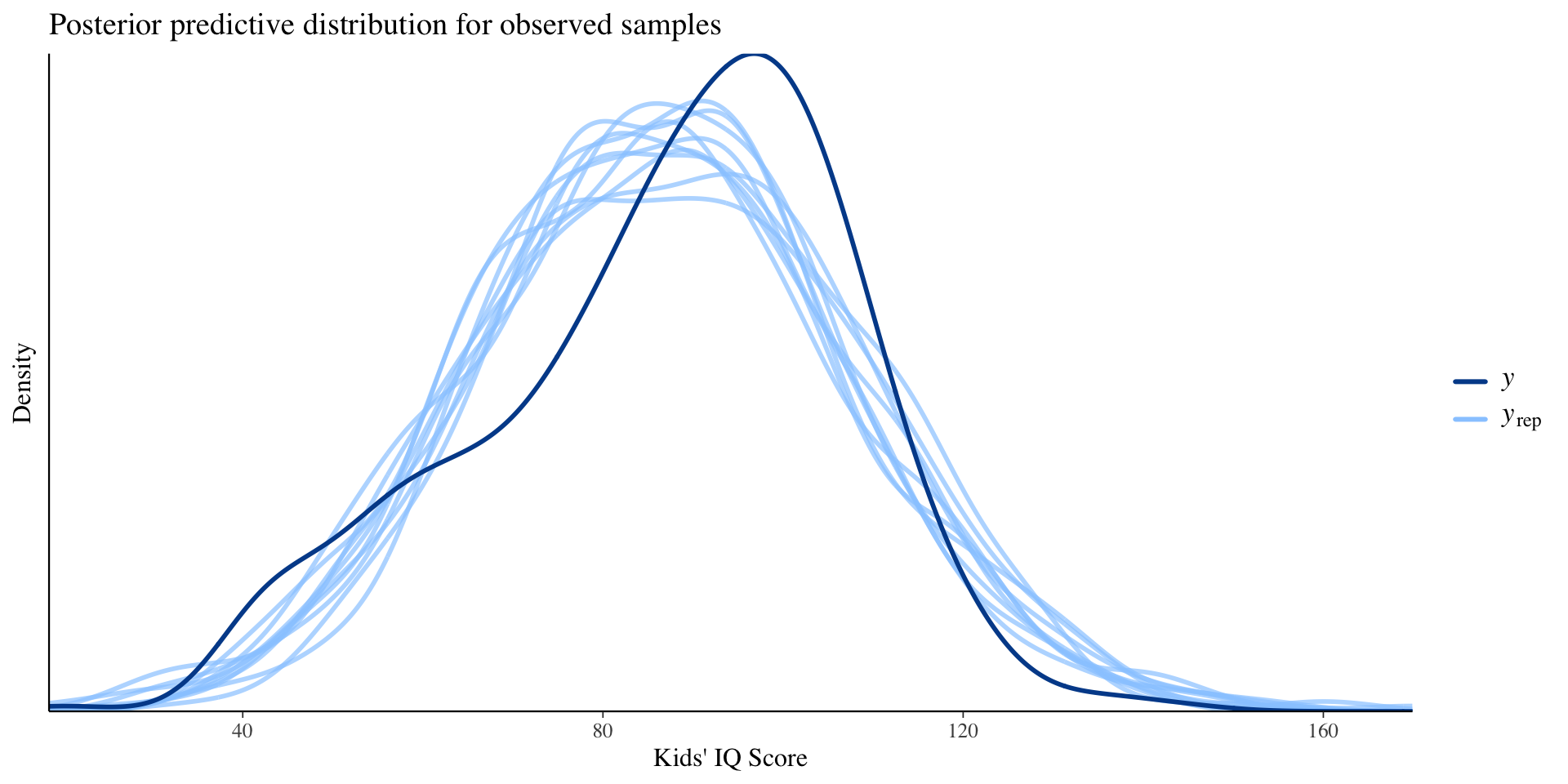
Posterior Prediction Checks (In-sample checking)

Compare observed data to draws from the posterior predictive distribution.

# predicted vs. observed
Y_rep <- posterior_predict(fit, seed = 2023)

ppc_dens_overlay(kidiq$kid_score, Y_rep[1:10,], size = 1) + 
  xlab("Kids' IQ Score") +
  ylab("Density") +
  labs(title = "Posterior predictive distribution for observed samples")

Posterior Prediction Checks (In-sample checking)

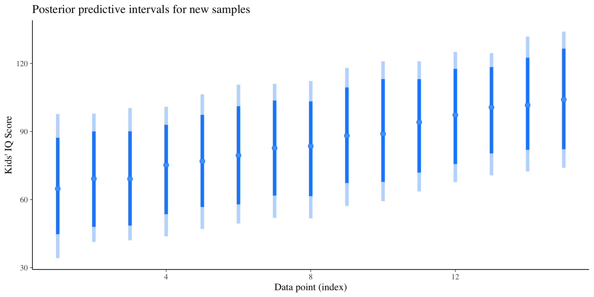
Posterior Prediction Distributions (Out-of-sample prediction)

Compute the posterior predictive distribution for a new sample.

X_new <- data.frame(mom_hs = 0, mom_iq = seq(70, 140, by = 5))
Y_new_pred <- posterior_predict(fit, newdata = X_new) 

ppd_intervals(Y_new_pred[1:500,], prob = 0.75, linewidth = 2) + 
  ylab("Kids' IQ Score") +
  ggtitle("Posterior predictive intervals for new samples")

Posterior Prediction Distributions (Out-of-sample prediction)

Interactive tool: `shinystan`

library(shinystan)
launch_shinystan(fit)

Regularized regression

Regularized linear regression

The OLS solution \(\hat{\beta} = (X^TX)^{-1}X^TY\) is obtained by minimizing the residual sum of squares (RSS), i.e., \(\arg\min_{\beta\in\R^p} \|Y - X\beta\|^2\).
In some cases, the matrix \(X^TX\) is ill-conditioned, i.e., the inverse \((X^TX)^{-1}\) is numerically unstable.
Also when \(p > n\), the matrix \(X^TX\) is singular and the OLS solution does not exist.
We can consider the following penalized least-square problem: \[ \arg\min_{\beta\in\R^p} \|Y - X\beta\|^2 + \lambda \cdot\text{Penalty}(\beta) \quad \text{for some } \lambda > 0. \]
There are three commonly used penalties:
- Ridge regression: \(\text{Penalty}(\beta) = \|\beta\|^2 = \sum_{j=1}^p \beta_j^2\)
- LASSO: \(\text{Penalty}(\beta) = \|\beta\|_1 = \sum_{j=1}^p |\beta_j|\)
- Elastic net: \(\text{Penalty}(\beta) = \alpha \|\beta\|^2 + (1-\alpha) \|\beta\|_1\) for some \(\alpha \in [0, 1]\).

Bayesian interpretation of regularization

Any penalized likelihood estimator has a Bayesian interpretation, i.e., it is the posterior mode under the prior \(\pi(\beta) \propto \exp(-\lambda\cdot\text{Penalty}(\beta))\).
For example,
- Ridge regression: normal prior \(\beta_j \sim N(0, \lambda^{-1})\)
- LASSO: Laplace prior \(\beta_j \sim \text{Laplace}(0, \lambda^{-1})\)
- Elastic net: \(\pi(\boldsymbol{\beta}) \propto \exp \left\{-\lambda_1\|\boldsymbol{\beta}\|_1-\lambda_2\|\boldsymbol{\beta}\|_2^2\right\}\)
Usually, the tuning parameter \(\lambda\) is chosen by cross-validation.
Under the Bayesian framework, we can
- put a prior on \(\lambda\) (fully Bayesian)
- put a hierarchical prior on \(\lambda\) (hierarchical Bayes)
- estimate it from the data (empirical Bayes)

Bayesian LASSO

LASSO = “Least Absolute Shrinkage and Selection Operator”
Model (this is how stan_glm implements LASSO prior): \[\begin{align*} Y \mid X, \beta, \sigma^2 & \sim N(X\beta, \sigma^2 I_n) \\ \beta_j & \iid \text{Laplace}(0, \lambda^{-1}) \\ \lambda & \sim \chi^2_{\nu} \end{align*}\] where \(\nu\) is the degrees of freedom (the default is \(\nu = 1\)).
Bias increases as \(\lambda\) increases (producing more zeroes).
Variance decreases as \(\lambda\) increases.
Hence larger value of \(\nu\) produces more shrinkage.

Bayesian LASSO

data <- read.csv("dataset/car_price/CarPrice_Assignment.csv")
fit_lasso <- stan_glm(price ~ highwaympg + citympg + horsepower + 
                          peakrpm + compressionratio, 
                      data = data, 
                      prior = lasso(df = 1, location = 0, 
                                    scale = 0.5, autoscale = TRUE),
                      prior_intercept = normal(location = 0, scale = 1, 
                                               autoscale = TRUE),
                      prior_aux = exponential(rate = 1, autoscale = TRUE),
                      chains = 4, iter = 2000, seed = 2023,
                      refresh = 0)

Summary of the fitted model


Model Info:
 function:     stan_glm
 family:       gaussian [identity]
 formula:      price ~ highwaympg + citympg + horsepower + peakrpm + compressionratio
 algorithm:    sampling
 sample:       4000 (posterior sample size)
 priors:       see help('prior_summary')
 observations: 205
 predictors:   6

Estimates:
                   mean    sd      10%     50%     90%  
(Intercept)       9493.2  4656.5  3681.0  9573.9 15322.0
highwaympg        -328.0   153.9  -528.2  -320.4  -140.2
citympg             71.7   171.2  -131.5    57.3   296.4
horsepower         139.0    12.4   122.9   139.2   154.7
peakrpm             -1.4     0.7    -2.3    -1.4    -0.5
compressionratio   451.8    88.6   338.3   450.3   564.1
sigma             4123.4   212.5  3858.6  4113.1  4398.4

Fit Diagnostics:
           mean    sd      10%     50%     90%  
mean_PPD 13262.4   398.9 12755.5 13256.9 13779.3

The mean_ppd is the sample average posterior predictive distribution of the outcome variable (for details see help('summary.stanreg')).

MCMC diagnostics
                 mcse Rhat n_eff
(Intercept)      72.0  1.0 4179 
highwaympg        2.6  1.0 3374 
citympg           2.9  1.0 3555 
horsepower        0.2  1.0 4133 
peakrpm           0.0  1.0 4251 
compressionratio  1.4  1.0 4222 
sigma             3.2  1.0 4291 
mean_PPD          6.4  1.0 3869 
log-posterior     0.1  1.0  801 

For each parameter, mcse is Monte Carlo standard error, n_eff is a crude measure of effective sample size, and Rhat is the potential scale reduction factor on split chains (at convergence Rhat=1).

High-dimensional linear regression

In some applications, we might have more predictors than samples, i.e., \(p \gg n\).
In such cases, the sparsity assumption is often used, i.e., only a few predictors are relevant.
LASSO or Bayesian Lasso can be used to select the relevant predictors.
However LASSO or Bayesian LASSO have some problems:
- it does not handle correlated variables well
- it shrinks all coefficients with the same intensity
- it often overshrinks large coefficients.
We will now introduce two priors for high-dimensional sparse linear regression that address these problems.

Spike-and-slab prior

The spike-and-slab prior¹ is \[ \beta_j \mid w, \tau^2 \sim (1 - w)\delta_0 + w \cdot N(0, \tau^2). \]
Equivalently, \[\begin{align*} \beta_j \mid \gamma_j = 0 & \sim \delta_0 \\ \beta_j \mid \gamma_j = 1 & \sim N(0, \tau^2)\\ \gamma_j & \iid \text{Ber}(w) \end{align*}\]
\(w\) is the parameter that controls the sparsity, and \(\gamma_j\) is the indicator of the \(j\)-th predictor being relevant.
This prior is considered the ``gold standard’’ for sparse regression.
However, it is computationally expensive to update the discrete variables \(\gamma_j\).

Horseshoe prior

The horseshoe prior¹ is \[\begin{align*} \beta_j \mid \lambda_j, \tau & \sim N\left(0, \tau^2 \lambda_j^2\right) \\ \lambda_j & \sim C^{+}(0,1), \quad j=1, \ldots, p \end{align*}\] where \(C^{+}(0, 1)\) is the half-Cauchy distribution.
This is an example of global-local shrinkage prior, where \(\lambda_j\) is the local shrinkage parameter and \(\tau\) is the global shrinkage parameter.

Available priors for `stan_glm`

Student-\(t\) family: cauchy, \(t\), normal
Hierarchical shrinkage family: horseshoe, horseshoe+
Laplace family: laplace, lasso
R2 prior: This prior hinges on prior beliefs about the location of \(R^2\), the proportion of variance in the outcome attributable to the predictors.
Check https://mc-stan.org/rstanarm/reference/priors.html for more details.

Compare different models

Suppose we have two regression models: \[\begin{align*} & Y = \beta_0 + \beta_1X_1\\ & Y = \beta_0 + \beta_1X_1 + \beta_2X_2. \end{align*}\]
We can compare these two models using the Bayes factor.
However, since we are fitting linear models, we can also use the \(R^2\) to compare the models.
The \(R^2\) statistic is defined as \[\begin{align*} R^2 & = \frac{\text{Explained variance}}{\text{Total variance}} = 1 - \frac{\text{Residual variance}}{\text{Total variance}}\\ & = 1 - \frac{\sum_{i=1}^n (y_i - \hat{y}_i)^2}{\sum_{i=1}^n (y_i - \bar{y})^2}. \end{align*}\]
Therefore, a model with a larger \(R^2\) is preferred.

Bayesian \(R^2\)

However, the \(R^2\) always increases even if we add irrelevant predictors.
Adjusted \(R^2\) is a modification of \(R^2\) that penalizes the addition of irrelevant predictors \[ R^2_{\text{adj}} =1-\left(1-R^2\right) \frac{n-1}{n-p-1}. \]
Instead of comparing the \(R^2\) or the adjusted \(R^2\) of the two models, we can compare the posterior distributions of the \(R^2\) of the two models.

Example

fit1 <- stan_glm(kid_score ~ mom_hs, data=kidiq, 
                 seed=2023, refresh=0)
fit2 <- stan_glm(kid_score ~ mom_hs + mom_iq, data=kidiq, 
                 seed=2023, refresh=0)

## Adding random noise as predictors
set.seed(2023)
n <- nrow(kidiq)
kidiqr <- kidiq
kidiqr$noise <- array(rnorm(5*n), c(n,5))
fit3 <- stan_glm(kid_score ~ mom_hs + mom_iq + noise, data=kidiqr,
                 seed=2023, refresh=0)

r2_fit1 <- bayes_R2(fit1)
r2_fit2 <- bayes_R2(fit2)
r2_fit3 <- bayes_R2(fit3)

Posterior distribution of \(R^2\)

Although adding noise predictors does increase the \(R^2\), the change is negligible compared to the uncertainty of \(R^2\).

Lecture 09: Bayesian Regression

Classical Linear regression

Linear regression

Normal linear model

Standard noninformative prior

Posterior distributions

Posterior predictive distribution

Computation

Example: Kids’ Test Scores1

Fit a Bayesian linear regression model

Summary of the fitted model

Prior Summary

MCMC Diagnostics

MCMC Diagnostic

Posterior Prediction Checks (In-sample checking)

Posterior Prediction Checks (In-sample checking)

Posterior Prediction Distributions (Out-of-sample prediction)

Posterior Prediction Distributions (Out-of-sample prediction)

Interactive tool: shinystan

Regularized regression

Regularized linear regression

Bayesian interpretation of regularization

Bayesian LASSO

Bayesian LASSO

Summary of the fitted model

High-dimensional linear regression

High-dimensional linear regression

Spike-and-slab prior

Horseshoe prior

Available priors for stan_glm

Compare different models

Bayesian \(R^2\)

Example

Posterior distribution of \(R^2\)

Example: Kids’ Test Scores¹

Interactive tool: `shinystan`

Available priors for `stan_glm`