Lecture 11: Gaussian Process

Chun-Hao Yang

Non-, Semi-, and Parametric Models

\[ \newcommand{\mc}[1]{\mathcal{#1}} \newcommand{\R}{\mathbb{R}} \newcommand{\E}{\mathbb{E}} \renewcommand{\P}{\mathbb{P}} \newcommand{\var}{{\rm Var}} % Variance \newcommand{\mse}{{\rm MSE}} % MSE \newcommand{\bias}{{\rm Bias}} % MSE \newcommand{\cov}{{\rm Cov}} % Covariance \newcommand{\iid}{\stackrel{\rm iid}{\sim}} \newcommand{\ind}{\stackrel{\rm ind}{\sim}} \renewcommand{\choose}[2]{\binom{#1}{#2}} % Choose \newcommand{\chooses}[2]{{}_{#1}C_{#2}} % Small choose \newcommand{\cd}{\stackrel{d}{\rightarrow}} \newcommand{\cas}{\stackrel{a.s.}{\rightarrow}} \newcommand{\cp}{\stackrel{p}{\rightarrow}} \newcommand{\bin}{{\rm Bin}} \newcommand{\ber}{{\rm Ber}} \DeclareMathOperator*{\argmax}{argmax} \DeclareMathOperator*{\argmin}{argmin} \]

• What we have learned so far are called parametric models, i.e., models that are determined by a finite number of parameters.
• Nonparametric models are models whose ``parameter’’ is infinite dimensional.
• Two common types of nonparametric models:
  • Nonparametric regression: \(Y = f(X) + \epsilon\), where \(f\) is an unknown function.
  • Nonparametric density estimation: \(X_1, \ldots, X_n \iid F\), where \(F\) is an unknown distribution (without assuming any parametric family).
• Semiparametric models are models that have both parametric and nonparametric components, e.g., \(Y = X^T\beta + f(Z) + \epsilon\).

Bayesian Nonparametrics

• For a nonparametric model, a Bayesian treats the unknown function/distribution as the parameter.
• Therefore, we need prior distributions for these parameters.
• We will introduce two “distributions” that are useful for nonparametric models:
  • Gaussian process (GP, the “distribution” of random functions)
  • Dirichlet process (DP, the “distribution” of random distributions)
• That is,
  • \(Y = f(x) + \epsilon\), \(f \sim \text{GP}\), \(\epsilon \sim N(0, \sigma^2)\).
  • \(X_1, \ldots, X_n \sim F\), \(F \sim \text{DP}\).

Why nonparametrics?

• Nonparametric models are more flexible than parametric models.
• Yet, nonparametric models are not always better than parametric models.
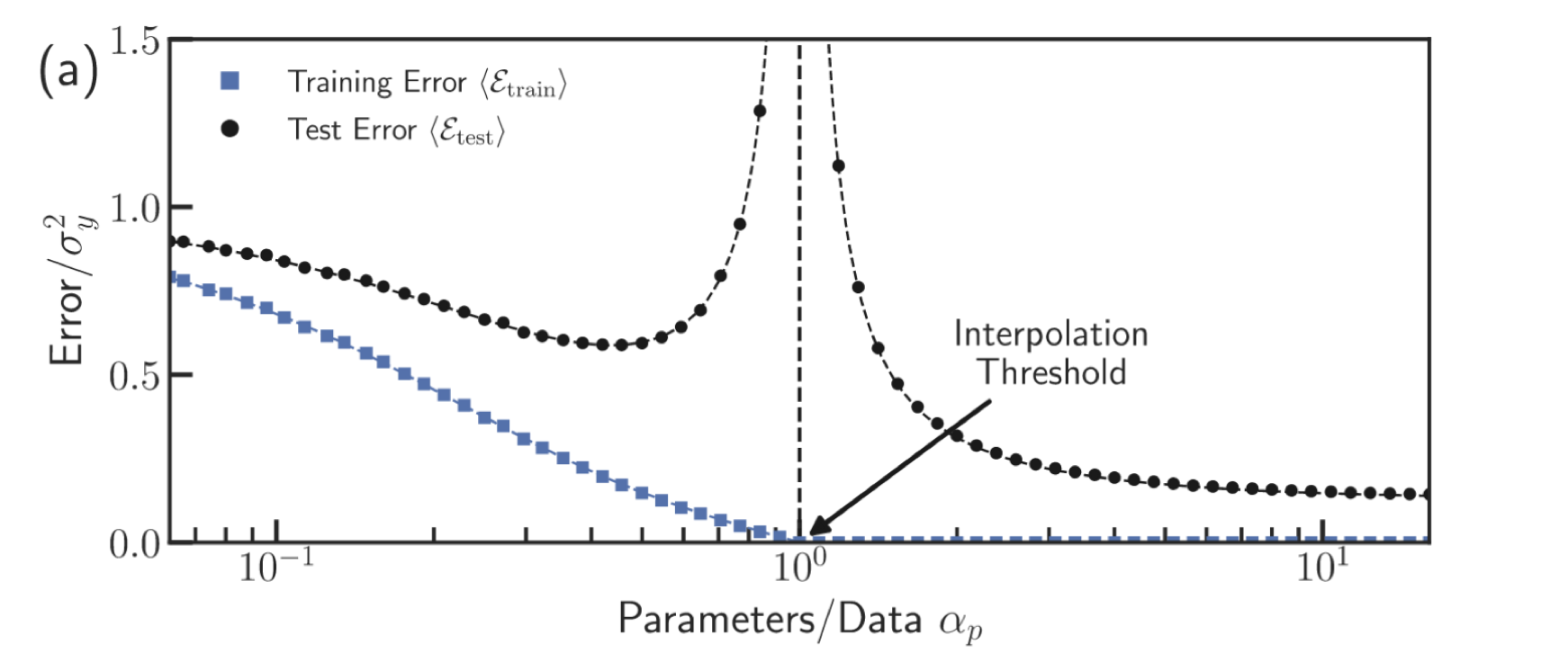
• As we increase the complexity of the model, we may
  • overfit the data;
  • increase the computational cost;
  • lose interpretability.

Double descent phenomenon

Image source: Shaeffer et. al. (2023)

Nonparametric regression¹

• Recall that a linear regression model assumes \(\E(Y \mid X) = X^T\beta\).
• A nonparametric regression model assumes \(\E(Y \mid X) = f(X)\), where \(f\) is an unknown function.
• There are different ways to estimate \(f\):
  • Kernel regression
  • Regression splines
  • Gaussian process regression
• For simplicity, we consider the one-dimensional regression problem, i.e., we have \(\{x_i, y_i\}_{i=1}^n\) where \(x_i, y_i \in \R\).
• The extension to higher dimensions is straightforward.

1. A good reference is this course note.

Kernel regression

• The Nadaraya–Watson kernel regression estimator of \(f\) is \[ \hat{f}(x) = \frac{\sum_{i=1}^n K_h(x - X_i) Y_i}{\sum_{i=1}^n K_h(x - X_i)}, \] where \(K_h(x) = K(x/h)/h\) is a kernel function, and \(h\) is a bandwidth parameter.
• That is, \(\hat{f}(x)\) is a weighted average of the \(Y_i\)’s, where the weights are determined by the kernel function \(K\).
• The kernel function \(K\) is usually chosen to be a symmetric density function, e.g., the standard normal density function.

Example

library(gplm) # for kreg()
set.seed(1)
n <- 1000
x <- rnorm(n)
y <- sin(x) + rnorm(n)
plot(x,y,col="gray")
curve(sin(x), add = T, col = "green")
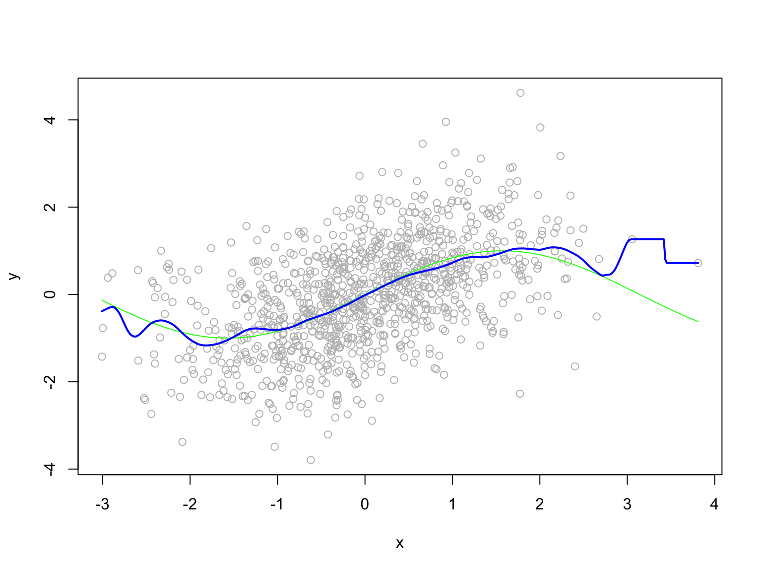
lines(kreg(x,y), lwd = 2, col = "blue")

Example

Regression splines

• A function \(g\) is called a \(k\)th order spline with knots \(t_0 < \cdots < t_m\) if
  • \(g\) is a polynomial of degree \(k - 1\) on the intervals \((-\infty, t_0], [t_0, t_1],\ldots, [t_m, \infty)\).
  • \(g\) has continuous derivatives up to order \(k - 2\) at each knot \(t_i\).
• Given a set of knots \(t_0 < \cdots < t_m\), the space of \(k\)th order spline has dimension \(m + k + 1\).
• There are many choices of basis for the space of splines. The most popular one is the B-spline basis.
• Hence a regression spline model is \[ \E(Y \mid x) = \sum_{j=1}^{m + k + 1} \beta_j B_j(x), \] where \(B_j\) is the \(j\)th B-spline basis function.

Regression splines

• Although a regression spline is determined by \(m+k+1\) parameters, it is usually referred to as a nonparametric model, since we are not interested in those parameters.
• The choice of knots is important.
• A smoothing spline uses all inputs as knots and avoids overfitting by shrinking the coefficients.
• A natural spline assumes polynomial of degree \((k-1)/2\) on \((-\infty, t_0]\) and \([t_m, \infty)\) to reduce variance at the boundary.
• Natural spline with cubic polynomial is the most common special case.

Example

Gaussian Process

Definition

A ``random function’’ \(f\) is said to follow a Gaussian process, denoted by \[ f \sim \mc{GP}(\mu, K), \] if for any \(x_1, \ldots, x_n\), the random vector \((f(x_1), \ldots, f(x_n))\) has a multivariate normal distribution, i.e., \[ \left[\begin{array}{c} f(x_1)\\ \vdots\\ f(x_n) \end{array}\right] \sim N\left(\left[\begin{array}{c} \mu(x_1)\\ \vdots\\ \mu(x_n), \end{array}\right], \left[\begin{array}{ccc} K(x_1, x_1) & \cdots & K(x_1, x_n)\\ \vdots & \ddots & \vdots\\ K(x_n, x_1) & \cdots & K(x_n, x_n) \end{array}\right]\right). \]

• The parameter \(\mu: \R \to \R\) is called the mean function.
• The parameter \(K: \R \times \R \to \R\) is called the covariance function/operator or kernel.
• The kernel \(K\) needs to be symmetric and positive definite, i.e, for any \(x_1, \ldots, x_n \in \R\), the matrix above is symmetric and positive definite.

Commonly used kernels

• Notation: for \(x, x^{\prime} \in \R^n\), \(K(x, x^{\prime})\) is an \(n \times n\) matrix whose \((i,j)\)th entry is \(K(x_i, x^{\prime}_j)\).

• Linear kernel: \(K(x, x^{\prime}) = x^Tx^{\prime}\).

• Polynomial kernel: \(K_{c,d}(x, x^{\prime}) = (x^Tx^{\prime} + c)^d\).

• Gaussian kernel: \(K_{\sigma}(x, x^{\prime}) = \exp\left(-\frac{\|x-x^{\prime}\|^2}{2\sigma^2}\right)\).

Simulating Gaussian processes

library(mvtnorm)
GP_sim <- function(from = 0, to = 1, mean_func = function(x){0},
                   cov_func = function(x1, x2){exp(-16*(x1-x2)^2)}, 
                   m = 500){
    x <- seq(from, to, length.out = m)
    mu <- sapply(x, mean_func)
    Sigma <- outer(x, x, Vectorize(cov_func))
    y <- rmvnorm(1, mu, Sigma)
    return(list(x = x, y = y))
}

Simulating Gaussian processes

Gaussian Process Regression

• Suppose we observe \(\{x_i, y_i\}_{i=1}^n\), \(x_i, y_i \in \R\).
• Let \(\mathbf{y} = [y_1, \ldots, y_n]^T\) and \(\mathbf{x} = [x_1, \ldots, x_n]^T\).
• Consider the model: \[\begin{align*} \mathbf{Y} \mid f, \mathbf{x}, \sigma^2 &\sim N(f(\mathbf{x}), \sigma^2I_n)\\ f \mid \mu, K &\sim \mc{GP}(\mu, K). \end{align*}\]
• The GP prior is equivalent to \(f(\mathbf{x}) \mid \mathbf{x}, \mu, K \sim N(\mu(\mathbf{x}), K(\mathbf{x}, \mathbf{x}))\).
• The likelihood is equivalent to \(\mathbf{Y} = f(\mathbf{x}) + \epsilon\), \(\epsilon \sim N(0, \sigma^2I_n)\).
• We need to compute two distributions:
  • The posterior distribution of \(f\) given \(\mathbf{y}\) and \(\mathbf{x}\).
  • The posterior predictive distribution of \(f(\mathbf{x}^{\prime})\) given \(\mathbf{y}\) and \(\mathbf{x}\).

Posterior Predictive Distribution

• The posterior distribution of \(f\) is also a Gaussian process \[ f \mid \mathbf{y}, \mathbf{x}, \sigma^2 \sim \mc{GP}(\bar{\mu}, \bar{K}) \] where \[\begin{align*} \bar{\mu}(\cdot) & = \mu(\cdot) + K(\cdot, \mathbf{x})[K(\mathbf{x}, \mathbf{x}) + \sigma^2I_n]^{-1}(\mathbf{y} - \mu(\mathbf{x}))\\ \bar{K}(\cdot, \cdot) & = K(\cdot, \cdot) - K(\cdot, \mathbf{x})[K(\mathbf{x}, \mathbf{x}) + \sigma^2I_n]^{-1}K(\mathbf{x}, \cdot). \end{align*}\]
• Hence the predictive distribution is a multivariate normal \[ f(\mathbf{x}^{\prime}) \mid \mathbf{y}, \mathbf{x}, \sigma^2 \sim N(\bar{\mu}(\mathbf{x}^{\prime}), \bar{K}(\mathbf{x}^{\prime}, \mathbf{x}^{\prime})). \]

Derivation

• For any \(m\) and \(\mathbf{x}^{\prime} \in \R^m\), \[ \left[\begin{array}{c} \mathbf{Y}\\ f(\mathbf{x}^{\prime}) \end{array} \right] \sim N\left(\left[\begin{array}{c} \mu(\mathbf{x})\\ \mu(\mathbf{x}^{\prime}) \end{array}\right], \left[\begin{array}{cc} K(\mathbf{x}, \mathbf{x}) + \sigma^2I_n& K(\mathbf{x}, \mathbf{x}^{\prime})\\ K(\mathbf{x}^{\prime}, \mathbf{x}) & K(\mathbf{x}^{\prime}, \mathbf{x}^{\prime}) \end{array}\right]\right). \]
• Therefore \[ f(\mathbf{x}^{\prime}) \mid \mathbf{y}, \mathbf{x}, \sigma^2 \sim N\left(\bar{\mu}(\mathbf{x}^{\prime}) , \bar{K}(\mathbf{x}^{\prime}, \mathbf{x}^{\prime})\right). \] where \[\begin{align*} \bar{\mu}(\mathbf{x}^{\prime}) & = \mu(\mathbf{x}^{\prime}) + K(\mathbf{x}^{\prime}, \mathbf{x})[K(\mathbf{x}, \mathbf{x}) + \sigma^2I_n]^{-1}(\mathbf{y} - \mu(\mathbf{x}))\\ \bar{K}(\mathbf{x}^{\prime}, \mathbf{x}^{\prime}) & = K(\mathbf{x}^{\prime}, \mathbf{x}^{\prime}) - K(\mathbf{x}^{\prime}, \mathbf{x})[K(\mathbf{x}, \mathbf{x}) + \sigma^2I_n]^{-1}K(\mathbf{x}, \mathbf{x}^{\prime}). \end{align*}\]
• That is, \(f \mid \mathbf{y}, \mathbf{x}, \sigma^2 \sim \mc{GP}(\bar{\mu}, \bar{K})\)

Example

Take \(n = 20\) and generate \(Y = \sin(X) + \exp(X/5) + \epsilon\) where \(\epsilon \sim N(0, 0.1^2)\).

Example

Fit a Gaussian process regression model with \(\mu(x) = 0\) and Gaussian Kernel.

library(GauPro)
gp <- GauPro(X, Y)
plot(gp)
curve(sin(x) + exp(x/5), -5, 5, add = TRUE, col = "red", lwd = 2)

Hierarchical Gaussian Process model

• In practice, there are other unknown parameters, for example \(\sigma^2\) or the hyperparameters in the kernel function.

• The hyperparameters in the kernel function can be selected via cross-validation.

• However, as a Bayesian, we can consider a fully Bayesian hierarchical model \[\begin{align*} \tau^2 & \sim \text{InvGamma}(c,d) \\ \sigma^2 & \sim \text{InvGamma}(a ,b) \\ f_i \mid x, \tau & \iid N(0, K(x, x\mid \tau) \\ y_i \mid f_i, \sigma^2& \ind N\left(f_i, \sigma^2\right) \quad i = 1, \ldots, n \end{align*}\] where \(K(x, y) = \exp\left(-\frac{(x-y)^2}{2\tau^2}\right)\).

• Additional priors can be assigned to the hyperparameters \(a,b,c\) and \(d\).

• The posterior distribution is \(\pi(f, \sigma^2, \tau^2 \mid \mathbf{y}, \mathbf{x})\).

Computational issues

• It seems that posterior computation in Gaussian process regression is trivial, but there are two main hurdles involved.
• The first hurdle is that the covariance matrix \(K(\mathbf{x}, \mathbf{x}\mid \tau^2) + \sigma^2I_n\) is \(n \times n\) and the computational complexity of the inverse matrix is \(O(n^3)\).
• This inverse matrix needs to be computed in each iteration of the MCMC algorithm, since we are also updating \(\sigma^2\) and \(\tau^2\).
• The second hurdle is that the posterior distribution is high dimensional, making the sampling inefficient.
• In this case, the posterior distribution is \((n + 2)\)-dimensional.
• There are some approaches to overcome these hurdles:
  • Marginalization
  • Approximation

Marginal likelihood GP

• If the data model is Gaussian, we can integrate over \(f\) analytically to get the log marginal likelihood for the covariance function parameter \(\tau^2\) and residual variance \(\sigma^2\) : \[\begin{align*} \log p\left(y \mid \tau^2, \sigma^2\right) & =-\frac{n}{2} \log (2 \pi)-\frac{1}{2} \log \left|K(x, x \mid \tau^2) + \sigma^2 I\right|\\ & \qquad -\frac{1}{2} y^{T}\left(K(x, x \mid \tau^2)+\sigma^2 I\right)^{-1} y \end{align*}\]
• Then we only need to sample from the posterior of \(\tau^2\) and \(\sigma^2\).
• With \(\tau^2\) and \(\sigma^2\), we can easily generate \(f\) from the posterior distribution, since it’s normal.

Latent Gaussian Process model

• We can also extend GP to non-Gaussian likelihoods, similar to GLM.
• That is, \[\begin{align*} Y \mid f, X, \phi & \sim F_{\theta, \phi}\\ \theta & = g^{-1}(f(X))\\ f & \sim \mc{GP}(\mu, K) \end{align*}\] where \(g\) is the link function and \(\phi\) is the dispersion parameter.
• For example, if \(Y\) is binary, we can use \[\begin{align*} Y \mid X & \sim \text{Ber}\left(\frac{\exp(f(X))}{1+\exp(f(X))}\right)\\ f & \sim \mc{GP}(\mu, K). \end{align*}\]
• Similar for the Poisson log-linear model.

Sum of Gaussian processes

• Gaussian processes can be directly fit to data, but more generally they can be used as components in a larger model. For example, \[\begin{align*} Y & = \sum_{i=1}^M f_i(X) + \epsilon\\ f_i & \ind \mc{GP}(0, K_i) \end{align*}\]
• Since the sum of normal is still a normal, the decomposition above is equivalent to the decomposition of kernel functions, i.e., \[\begin{align*} f \sim \mc{GP}(0, \tilde{K}), \quad \tilde{K} = \sum_{i=1}^M K_i. \end{align*}\]

Example: Decomposing the time series

• The dataset contains records of all births in the United States on each day during the years 1969–1988.
• Additive model: \[ y(t)=f_1(t)+f_2(t)+f_3(t)+f_4(t)+f_5(t)+\epsilon_t, \] where \(y(t)\) is the number of births on day \(t\).
• The components \(f_i\) represent variation with different scales and periodicity

This example is from BDA Ch. 21.2.

Example: Decomposing the time series

1. Long-term trends: \(f_1(t) \sim \operatorname{GP}\left(0, k_1\right), \quad k_1\left(t, t^{\prime}\right)=\sigma_1^2 \exp \left(-\frac{\left|t-t^{\prime}\right|^2}{2 l_1^2}\right)\)
2. Short-term variation: \(f_2(t) \sim \operatorname{GP}\left(0, k_2\right), \quad k_2\left(t, t^{\prime}\right)=\sigma_2^2 \exp \left(-\frac{\left|t-t^{\prime}\right|^2}{2 l_2^2}\right)\)
3. Weekly quasi-periodic pattern: \(f_3(t) \sim \operatorname{GP}\left(0, k_3\right), \quad k_3\left(t, t^{\prime}\right)=\sigma_3^2 \exp \left(-\frac{2 \sin ^2\left(\pi\left(t-t^{\prime}\right) / 7\right)}{l_{3,1}^2}\right) \exp \left(-\frac{\left|t-t^{\prime}\right|^2}{2 l_{3,2}^2}\right)\)
4. Yearly smooth seasonal pattern: \(f_4(t) \sim \operatorname{GP}\left(0, k_4\right), \quad k_4\left(s, s^{\prime}\right)=\sigma_4^2 \exp \left(-\frac{2 \sin ^2\left(\pi\left(s-s^{\prime}\right) / 365.25\right)}{l_{4,1}^2}\right) \exp \left(-\frac{\left|s-s^{\prime}\right|^2}{2 l_{4,2}^2}\right)\) where \(s = t \text{ mod } 365.25\)
5. Special days including an interaction term with weekend: \(f_5(t)=I_{\text {special day }}(t) \beta_a+I_{\text {weekend }}(t) I_{\text {special day }}(t) \beta_b\)
6. Unstructured residuals: \(\epsilon_t \sim N\left(0, \sigma^2\right)\)

Example: Decomposing the time series

Example: Decomposing the time series

Example: Decomposing the time series

• This model can be improved by further decomposing the time series.
• For example, assume that the effect pf special day will change over time.

Other applications of GP

There are many other applications of GP:

• Functional data analysis: the observed data are functions
• Spatial data analysis: the data has spatial (location) characteristics
• Density estimation:
  • Assume the unknown density to be \(p(x \mid f) = \frac{\exp(f(x))}{\int \exp(f(x^{\prime})) dx^{\prime}}\) and \(f \sim \mc{GP}(\mu, K)\).